Mixed effects: Introduction#
Note: This is not intended to be a full treatment of mixed effects, and this tutorial assumes you have some exposure. It does review a few key concepts, however.
Mixed effects models extend the idea of GLS to more complex error structures. In particular, errors can be correlated because they belong to the same group. Groups can include multiple measures taken from the same:
Participant: e.g. trials in a psychology study, or time points in a physiological study (e.g., fMRI)
Geographic area: e.g., zip code, in epidemiological or political studies
Item: e.g., individual pictures, words, or other stimuli in a psychology experiment
Family: e.g., twins or extended family members
Cohort: e.g., the same group in a group therapy study
Time frame: e.g., day, if multiple participants are tested on a given day
Experimenter: e.g., therapist, nurse, or other experimental personnel
In some cases we are interested in the variation across specific levels of these and other experimental variables. In other cases, we would like to generalize across levels of these variables. For example, in a marketing study, we may be interested in the difference between two specific items, Advertisement A vs. B. We may test participants in groups, and we would like to generalize across the groups to the population of people exposed to the ad at large. In this case, quantifying the uncertainty (i.e., error variance) so that we can have an appropriate level of confidence in generalizing to new groups requires accounting for the possibility that there may be a random effect of the particular group in which a person is tested.
As with any GLM, we would like to estimate and make inferences about the population values of some fixed effects. Fixed effects are those for which differences across the levels of the specific variables tested are meaningful to us. e.g.:
Drug: Prozac vs. placebo
Sex: Male vs. female
Item: Advertisement A vs. B
We model these in the design matrix, \(X\).
Effects whose levels we would like to generalize over when making inferences on the fixed effects must be modeled in the error structure, \(\Sigma\). These are random effects. We estimate parameters for variance components–generally, one for residual variance \(\sigma^2\) and a series of parameters reflecting the variances and covariances across observations from the same group. In the example above, Item would be modeled as fixed (estimated with \(\hat\beta\)), and Group would be random (estimated with \(\hat{U}\) below).
\(\Sigma\) is structured so that errors on observations from the same groups may be correlated. In the OLS case, \(\Sigma=\sigma^2I\). In the general mixed effects case, the diagonal elements may be unequal across blocks of observations, reflecting different error variances across different groups or subsamples. The off-diagonal elements will reflect error covariance among observations collected from the same groups. We model this structure by estimating parameters reflecting these covariances.
Within- and between-person effects#
In psychology and neuroscience experiments (and many other types of studies), it is very common to collect multiple observations from the same individuals. It is also common to manipulate and/or test effects that vary within-person, e.g., an experimental manipulation of a factor where each person experiences all the levels of a factor. These are within-person effects. Examples include:
Multiple levels of experimental pain intensity administered within-person
Difficult and easy math questions assessed within-person
Repeated measures across time: Participants are assessed pre- and post-intervention (as with the Ashar dataset)
Treatment (in a crossover design, in which each person experiences each treatment)
Age (in a longitudinal study)
These effects would usually be treated as fixed effects. If each person experiences each level of the effect, they are said to be crossed with person. In rare cases, e.g., people sampled over multiple years but at different ages, or with missing data, they may not be fully crossed.
Other things being equal, within-person effects have much lower error variances and are much less susceptible to confounds, because they eliminate many sources of variability among people that can influence the observations. With such effects, “Each person serves as their own control”. Fully crossed designs are also the most powerful.
Another class of variable is assessed only at the person-level, with one value per person. These are between-person variables. Examples include:
Patient status (patient or control)
Treatment (in a parallel groups design, in which each person experiences only one treatment)
Age (in a cross-sectional study)
Sex
These effects would usually be treated as fixed effects. People are nested within these effects, since each person experiences or belongs to only one level of the variable.
Together, these two kinds of effects can be thought of as organized in a hierarchy, with the 1st level reflecting within-person effects, and the 2nd level reflecting between-person effects. The intercept at the 2nd level reflects the expected (average) within-person observation when all 2nd-level (between-person) predictors are at 0.
Crossed and nested random effects#
If lower-level effects are nested within or crossed with a random effect (e.g., participant), we need to specify that the errors are grouped by that random effect.
Here are some common structures:
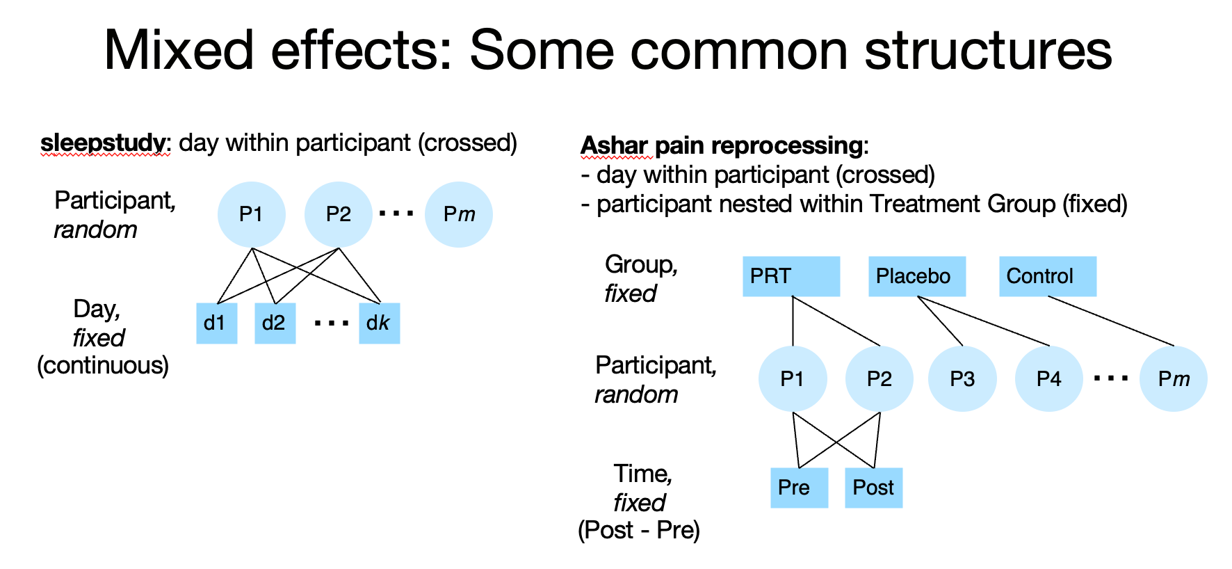
In the sleepstudy dataset, day (fixed) is measured within-participant. These are crossed, because each participant is measured on each day. We would model this in Wilkinson notation with the term (day | participant).
In the Ashar pain dataset, time (fixed) is measured within-participant (Pre- vs. Post treatment scores). Time is crossed with participant, because each participant is measured at each time. Group (3 levels, fixed) is between-participant, as each participant belongs to only one group. We are most interested in the Group x Time interaction (or, perhaps better, the effect on Post controlling for Pre). The errors on the Group effect are not grouped by participant, but the errors on Time are. We would therefore model Group with only fixed effects, and time grouped by the random participant effect. In Wilkinson notation: Group + Time + Group x Time + (Time | participant).
Random effects can be crossed or nested as well. Below, Items (e.g., emotional pictures) are nested within Valence (negative or positive for simplicity, but this could be a continouous variable as well). If we are interested in generalizing to new Items, we should model item-related variance as a random effect.
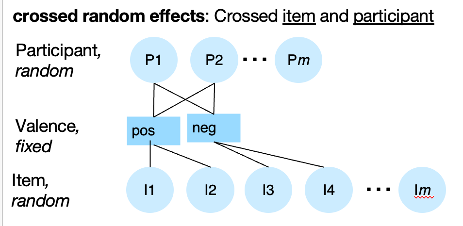
If each Item I1…Ik is measured for each person, Item and Participant are crossed. We would indicate that with separate random effects: Valence + (Valence | participant) + (1 | Item). This means that each unique items has its own item-level mean estimate in the model, and the Item-level variance is independent of the Participant-level variance.
However, if each Item I1…Ik is measured on only ONE person, so that different participants see different items, Item and Participant are nested. We would indicate that with a nested random effects: Valence + (Valence | participant/item). However, if you do not have multiple measures on each item, you cannot estimate such a model, because you can’t separate item-level variance from residual error variance.
Designs can have combinations of crossed and nested random and fixed factors.
Here are some more examples, from Krzywinski 2014 Nature Methods:
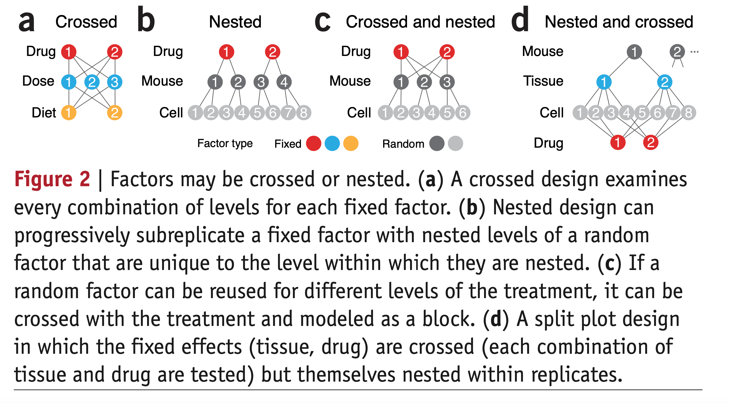
This schematic uses mouse instead of person, but the same principles apply. We always want to model mouse as a random effect. Unique cells assessed are also a random factor. If we assess each cell only once, we don’t need to model cell as a random effect explicitly; no errors are grouped by cell if there is only one observation per cell. But if we assess each cell multiple times through “technical replicates” (multiple tests of an assay), yielding multiple observations per cell, then we must include Cell as a random effect nested within Mouse.
(a) Has only fixed factors. This would be a design in which different animals are used in different combinations of treatments. Our model would have fixed effects of Drug * Dose * Diet (the 3-way interaction implies all main effects and pairwise interactions are also estimated). These are included automatically. As diagrammed, only one cell is assessed and there are no “technical replicates”, so there are no random effects.
(b) Is a “parallel groups” design in which different mice are tested on each of 2 drugs. We’d model Drug + (1 | Mouse). Errors are grouped by mouse (with multiple observations per mouse), but Drug is not assessed within-mouse (i.e., crossed with mouse). If there is only one measurement per cell, we do not need to model Cell as a random effect, because no errors are grouped by Cell. However, if we have technical replicates, we would model Cell as a random effect as well, in which case we would have nested random effects. We’d model Drug + (1 | Mouse/Cell). The random effects include an intercept only, because we do not have Drug effects varying within-Mouse or within-Cell (i.e., Drug and Mouse are not crossed), so we cannot estimate the Drug x Mouse interaction or Drug x Cell interaction.
(c) Is a “within-participant crossover” design, where Drug is crossed with Mouse. We would model this Drug + (Drug | Mouse). This models the Drug x Mouse interaction (the differences in Drug effect across individual levels of Mouse) and includes it in the error term. Equivalently, we can say that it estimates the error variance in the slope of Drug (Drug effect) across mice.
Including (Drug | Mouse) implies a random intercept term as well, which is included automatically. Thus, this is equivalent to (1 + Drug | Mouse).
Most models will also include error covariance terms for the random effects terms as well. Here, this means that the variances across individual mice in the intercept (1) and slope (Drug) may be correlated, and the mixed effects model estimates cov(intercept, Drug). If we wanted to explicitly assume uncorrelated random effects, we would separate the terms like so: (1 | Mouse) + (0 + Drug | Mouse).
If there are technical replicates, i.e., multiple observations per cell, we’d model both the random effects crossed with Drug and the nested structure, i.e., Drug + (Drug | Mouse/Cell).
(d) Tests different drugs on different cells extracted from 2 tissues. Drug and Tissue are fixed because we are interested in these specific drugs and tissues (not generalizing to new ones). All effects are crossed with Mouse, so we’d do Tissue * Drug + (Tissue * Drug | Mouse)
!Important! In all the cases with random effects above, if we ignore the random error structure, we will (a) not estimate the error variance correctly, and (b) not adjust the degrees of freedom correctly. This invalidates statistical inferences made on fixed effects. More detail is below.
Here is a guide to Wilkinson notation for a number of common structures:
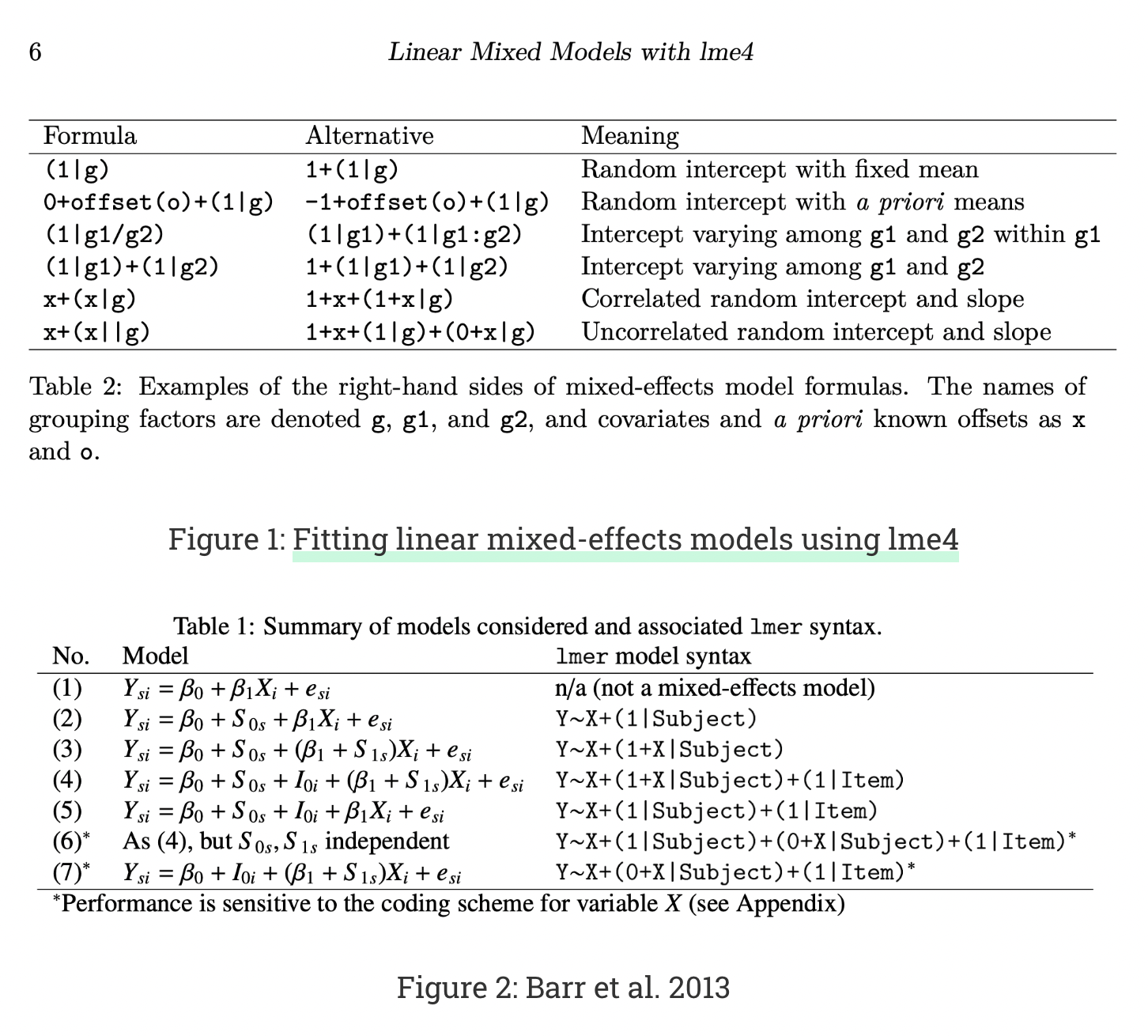
This page on Wilkinson notation is also really helpful!
For more on crossed and nested random effects, see Krzywinski 2014 Nature Methods
the Clapham mixed effects video on Youtube:

Two-stage summary statistics and mixed effects#
Let’s see how this maps onto the Ashar clinical trial dataset.
What we have done so far with the Ashar dataset is a version of a mixed effects model. It is a two-stage summary statistics approach.
Time (Post vs. Pre-treatment) is a within-person (1st-level) variable. Group (PRT vs. Placebo vs. Control) is a between-person (2nd-level) variable. Pain (BPI) is the outcome or DV.
Previously, we used two approaches:
We estimated a difference score, Post - Pre-treatment Pain, for each individual. This is a within-person contrast. Then, we used a GLM to assess the effect of Group (2 regressors) on the difference scores. The F-test for Group corresponds to a one-way ANOVA on improvement scores by Group, and we coded the 2 regressors for Group to estimate specific contrasts of interest (PRT - Placebo, mean(PRT + Placebo) - Control).
We analyzed Group differences in Post-treatment scores (the pain measure expected to show a group difference) controlling for Pre-treatment Pain. This entailed including regressors for Group (as above) and a continuous covariate for Pre-treatment Pain.
The data were organized in a “wide format” table, with only one row per participant. Therefore, when we ran the analyses above, \(y\) was always an \([m x 1]\) vector with 1 value for each of \(m\) participants. Assuming participants’ errors are uncorrelated, the OLS approach is valid.
The difference scores are contrast values, with a [1 -1] contrast across the within-person variable Time (pre vs. post)
The group membership (PRT, Placebo, Control) is a between-person variable, because each person has only one value.
Therefore, we used contrasts to estimate summary statistics for each person that capture the within-person effects, and analyzed the between-person effects on those difference scores using a single-level GLM. This corresponds to testing the [Group x Post vs. Pre-treatment] interaction.
Another way to do this is using a mixed effects model. Instead of organizing data in a “wide format” table with one row per participant, we can use the “long format” table, in which \(y\) (i.e., Pain) is an \([mk x 1]\) vector with \(k\) values measured for each of \(m\) participants. We model the correlation between within-person repeated measures (Pre and Post-treatment pain) by including a random effect of participant in the error model.
We explore that in the next module.
Degrees of freedom in mixed models#
Most mixed models do not usually directly estimate the individual participants’ predictions (or, more generally, individual level effects for any random effect). Instead, they estimate the variances across levels of those predictions, and use generalized least squares (GLS) to decorrelate the error and estimate the error degrees of freedom (dfe). (The dfe is debated, and some packages like lmer decline to estimate degrees of freedom).
Two ways to obtain P-values for fixed effects are:
Use the Satterthwaite approximation to estimate the dfe. For within-person variables crossed with a random effect of participant, these should usually be close to the number of participants. The same holds for effects nested within or crossed with a random effect.
Use model comparison with a likelihood ratio test to compare models with and without a fixed effect of interest (but keeping the random effects in the reduced model).
Satterthwaite#
Given the hat (projection) matrix:
The equation for the Satterthwaite approximation in general is:
% Matlab code
H = X * inv(X'*X) * X';
dfmodel_Satt = trace(H'*H)^2/trace(H'*H*H'*H) % Degrees of freedom for the column space (model)

R = eye(size(H)) - H;  % Residual-inducing matrix
For the error df, or dfe, we need to calculate the residual-inducing matrix:
Then, the Satterthwaite approximation for dfe is:
Given a known autocorrelation matrix \(V\), the GLS solution for \(H\) and \(R\) are:
The equation for the Satterthwaite approximation of dfe is:
Note: These last equations need further checking.
This is a general form for the degrees of freedom based on the residual-inducing matrix and variance components. Note, the exact computation can vary based on the specific model and its assumptions.
% Matlab code
% Simulate a known autocorrelated error structure (AR(1))
c = 0.5.^[0:size(X, 1)-1];  % autocorrelation matrix V under ar(1) with rho = 0.5
V = toeplitz(c);
figure; imagesc(V)

H = X * inv(X'*inv(V) * X) * X' * inv(V);   % Hat matrix
R = eye(size(H)) - H;                       % Residual-inducing matrix
dfe_Satt = trace((R*V)'*(R*V))^2/trace((R*V)'*(R*V)*(R*V)'*(R*V)) % Error degrees of freedom
Shrinkage in mixed models#
Most mixed models do not explicitly identify effects for individual levels of random effects (e.g., slopes for individual participants) in the course of model estimation. All that is required for statistical inference is to estimate their variances and the associated reduction in degrees of freedom for the fixed effects.
It is possible to obtain individual slope values. These are often called the Best Linear Unbiased Predictors (BLUPs), or in lmer, Conditional Modes (CM, modal random effect levels conditional on fixed population effects).
The BLUPs/CMs shrink the individual estimates towards the population means in proportion to the variance (inverse precision) of each level of the individual level estimates. For example, they would shrink individual participant slope estimates by the variance for each individual participant when modeling participant as a random effect). In the rest of the discussion below, we use participant to illustrate levels of a random effect, but the same principles apply to all types of random effects (e.g., items, cells, etc).
More precisely, the variance of an individual level (e.g., person’s) estimate (e.g., slope) is the sum of the between-person variance for a given effect \(i\), \(\sigma^2_{b, i}\) and within-person variance \(\sigma^2_{w, i}\). Note these are not residual variances, but variances of regression slopes \(i={1...I}\).
\(\sigma^2_{b, i}\) depends on the true inter-person variation in effects. People will differ no matter how much data is collected per person.
\(\sigma^2_{w, i}\) depends on:
The within-person design matrix \(Z\). Some effects are estimated more precisely than others.
The amount of data collected for that individual person (factored into \(Z^TZ\))
Other sources of error that affect some participants more than others (heteroscedasticity).
The residual variance \(\sigma^2\) and other correlated errors built into the within-person covariance matrix \(V\).
In practice, some packages like lmer (in R) ignore (3) above and assume equal error variances across all participants.
As shrinkage for is proportional to \(\sigma^2_{b, i} + \sigma^2_{w, i}\), the individual-level BLUP or CM is a weighted average of population-level and individual-level estimates, with weights for effects \(i={1...I}\) equal to:
As \(sigma^2 \to 0\), the individual estimate becomes very precise, and \(w \to 1\). As \(U_g \to 0\), \(w \to 0\), and all BLUPs are the population-level estimates. With equal within-person and population-level (random effects) variance, \(w = 1/2\).
Note: This section needs further checking for accuracy and completeness.
Don’t ignore random effects#
An important rule of thumb is that if we want to generalize to new, unobserved levels of a variable (e.g., participant), we must (1) estimate the variance across levels of the variable appropriately, (2) include that variance in the error term inferential test statistics (i.e., t- and F-tests), and (3) adjust the degrees of freedom appropriately.
If you ignore a random effect (e.g. of participant), then you will not do any of the three things above. If you model participant as a fixed effect (i.e., create a set of regressors that capture all differences across participants), you will still not be doing any of those critical things.
If you do not model an effect as random, you will not be able to generalize to unobserved levels. For example, imagine you conduct a study of differences in brain activity for negative vs. positive words. You collect fMRI activity while participants read 10 positive words and 10 negative words (a within-person factor). If you do not model word identity as a random effect, you will not be able to generalize to new words! That is, your conclusions might hold for the specific words you chose, but not different words.
Is this a problem? Generally, yes. You’re likely going to make conclusions about “positive words” as a class, but your statistical inferences can’t support that generalization. Thus, the idea of “keeping it maximal” and modeling random effects that exist in your study structure is usually a good idea.
!Important! In all the cases with random effects above, if we ignore the random error structure, we will (a) not estimate the error variance correctly, and (b) not adjust the degrees of freedom correctly. This invalidates statistical inferences made on fixed effects.
Testing the significance of random effects requires obtaining P-values for whether the random effects variance is different from 0. This amounts to testing whether there are individual differences across levels of random factors like Subject, Mouse, or Cell above. This is sometimes done with F-tests, but their performance is poor. Likelihood ratio tests excluding the random effects is a more well-accepted approach.
Just because you do not detect a “significant” random effect, it does not mean you can exclude it from the model. Such tests are not very inaccurate and subject to low power in many cases. As with all classical significance tests, the lack of a significant effect does not demonstrate that no effect exists – just that you cannot detect it with enough confidence. Therefore, do not test the signficance of your random effects and omit them from the model if they are non-significant. You will mis-estimate the error variance and dfe, and make invalid inferences.
Know when not to model an effect as random#
A very common situation in psychology and neuroscience is to measure only a few levels of a variable. You might measure “hard” and “easy” math problems, or 3 levels of pain, or 8 body sites. Do you want to generalize to other levels? You might, but you can’t. For example:
You can’t say that a training intervention affects performance on math problems that are harder or easier that those you tested.
You can’t say that a drug treatment affects pain responses to stimulus intensities or a body site you didn’t test.
In some cases, it doesn’t really make sense to think of these variables as drawn at random from a population. There’s not an infinite population of pain intensity levels or difficulty levels – there’s a continuum. And unlike participants, which we assume we can sample at random, intensity levels are not interchangeable for one another. The generalizability issue comes down to the question of whether the effects hold beyond the range of conditions under which you tested them. Thus, a solution is to sample a reasonable range and be careful not to extend inferences to levels far outside of that range. In this situation, you’d model intensity and difficulty levels as fixed effects, or (if more levels are included) treat them as continuous fixed effects.
Likewise, there is not an infinite population of body sites, and body sites are not interchangeable. It’s most appropriate to model body site as a fixed effect, and sample a range of disparate body sites. If an effect holds for some locations tested on arms, legs, head, and torso, it likely holds for other nearby ones as well. Of course, this can go wrong, and we should always consider that we don’t know the boundary conditions on generalization of effects.
Judd et al. 2012 showed that when you have crossed random effects of item and subject, the power is limited by the smaller of the two. If you have 1 million participants but only a small number of items, you will never be able to generalize to new items with high power! In this case you must either choose a different way to generalize, or re-design your study to include more items! By a “different way to generalize”, we mean:
Replicate the study using a different set of items
Make and validate predictions for new (untrained) items

More generally, I’m not sure it’s a great idea to ask your P-values to do all the generalization work for you. There will always be boundary conditions that it is difficult to test, and certainly difficult to sample broadly enough to include them as random effects in a mixed effects model. Experimenter, set and setting (testing location), time of year, population, paradigm design features, etc., etc. are all potential boundary conditions that could lead to a failure to generalize. We need to see which effects are robust across variations in these.
Replication across different variants can be more convincing than a low P-value in a table.