6. Inferences About Mind, Brain, and Behavior: The Statistical Brain Mapping Approach
Inferences About Mind, Brain, and Behavior: The Statistical Brain Mapping Approach
Run this code: ⚡ In-browser lab · Colab · MATLAB Online
Overview
Nearly every colorful brain image you have seen — in a journal, a news story, or a courtroom — is a statistical construction. The colored blobs do not show brain activity directly. They show the results of hypothesis tests performed across brain voxels, color-coded by the strength of the evidence that some effect — a response to a task, a correlation with behavior — is different from zero. This practice, called statistical parametric mapping (or mass-univariate analysis, or simply brain mapping), underlies the vast majority of images in scientific publications and popular media. Understanding what such maps can and cannot tell us is essential for scientists and non-scientists alike.
The first question to ask about any brain map is what effect it depicts. Researchers map many kinds of relationships onto local brain regions: effects of experimental manipulations (e.g., a [Task − Control] comparison), correlations with behavior or clinical status, trial-by-trial associations, decoding accuracy, functional connectivity with other regions, and network properties such as hub status. The second question is to whom the map applies. Single-subject maps are built from one person’s data — for example, by statistically comparing the time series measurements from a task condition against a control condition at each voxel. They are valuable in vision science, presurgical mapping, and clinical applications, but they cannot tell us how brains work in general. Group-level maps are needed for population inference: typically, a [Task − Control] difference image is computed for each participant, and then a second statistical test at each voxel asks whether the effect is consistent enough across people to generalize to the population — treating participants as a random effect.
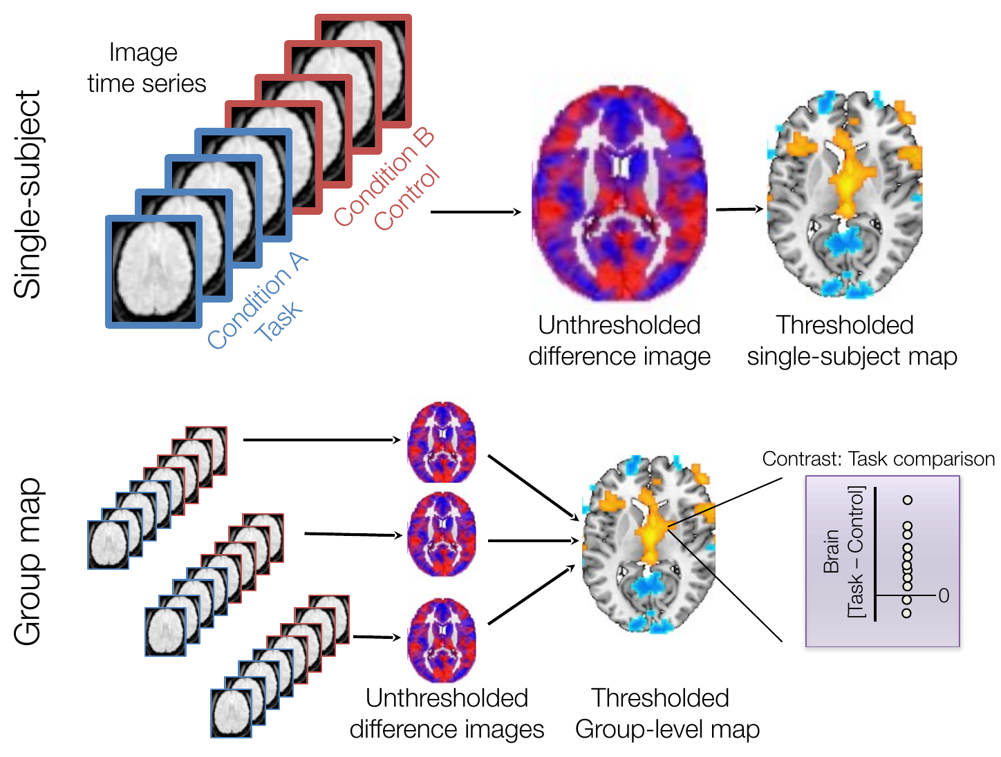
Single-subject and group-level statistical maps. Top: a statistical test of the [Task − Control] difference is performed on the time series from each voxel, giving an unthresholded map that is thresholded for interpretation. Bottom: one unthresholded difference image per participant is carried to a group analysis, and voxels whose group effect differs significantly from zero appear in the thresholded group-level map. (Figure 6.2 from the book. © the authors and MIT Press; reproduced with permission — not covered by this site’s CC-BY license.)
How is a map constructed? It helps to consider the generative process we assume. An exogenous variable of interest — say, an experimental task — causes a change in activity in some brain areas. We cannot observe this true signal; it is mixed with stochastic noise, and only the mixture is observed. The analysis aims to identify voxels containing true non-zero effects, using a separate hypothesis test at each voxel. The test statistic divides the estimated effect magnitude, written (often in units of percent BOLD signal change), by its standard error — a measure of how much the estimate would vary from sample to sample by chance:
t — test statistic at one voxel · β̂ — estimated effect magnitude (e.g., % BOLD signal change) · SE(β̂) — estimated standard error of β̂
where is the test statistic computed separately at each voxel, the estimated effect magnitude, and its estimated standard error — the expected sample-to-sample variability of under noise alone.
The null hypothesis at each voxel is that the true effect is zero. If we are willing to make some assumptions, the t-statistic has a known probability density function under the null, so we can compute a P value — the probability of observing a statistic as or more extreme if there were truly no effect. With 30 participants, for example, there is a 10% chance of observing even when the true effect is exactly zero, so yields and would not pass a conventional threshold, where is the pre-set acceptable false positive rate (the Type I error rate). Crucially, “non-significant” does not mean we should be certain there is no effect — and a significant voxel licenses only the claim that some non-zero effect exists there, not that the effect is large or meaningful.
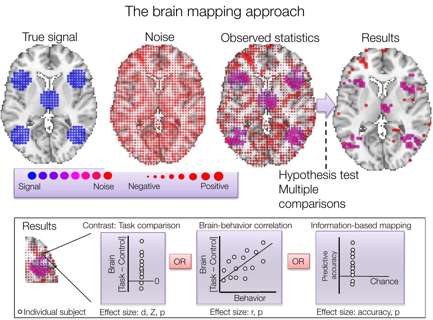
The brain mapping framework. Signal (blue) and noise (red) combine additively; the statistical evidence for true signal is evaluated in each voxel, a threshold is applied (with correction for multiple comparisons), and supra-threshold regions are interpreted anatomically. Some surviving voxels contain true signal mixed with noise; others are pure false positives. Bottom: effects commonly mapped voxel-wise include task comparisons, brain–behavior correlations, and local decoding accuracy. (Figure 6.4 from the book. © the authors and MIT Press; reproduced with permission — not covered by this site’s CC-BY license.)
Because a whole-brain analysis performs up to ~330,000 tests, using at each voxel would produce thousands of false positives. Brain mapping therefore uses much more stringent thresholds that control either the family-wise error rate (the chance of any false positive voxel across the whole family of tests) or the false discovery rate (the expected proportion of “significant” voxels that are false positives). When P values come from comparing statistics like t against their canonical assumed distributions, we are using parametric statistics; nonparametric alternatives such as permutation and bootstrap tests compute P values from the data themselves, at the price of more computation but fewer assumptions.
Voxel-wise mapping is not the only option. The earliest imaging studies instead averaged signal within predefined regions of interest (ROIs) and performed a single test. Whole-brain mapping and single-ROI testing are opposite ends of a continuum of multiple testing. Voxel-wise maps require little prior anatomical commitment and can reveal unexpected findings — but stringent correction reduces power, and selecting significant voxels inflates their apparent effect sizes. A single a priori ROI maximizes power and avoids selection bias — if the hypothesis is right; even a slightly misplaced ROI can miss a real effect entirely. In between lie sets of ROIs, or voxel-wise tests within ROIs. The advantages of prior specification hold only if ROIs were truly chosen a priori and all tests are reported: adjusting “a priori” regions after seeing results, or trying many analyses and reporting the best, are forms of P-hacking and HARKing that produce significant-looking results even when no true effect exists.
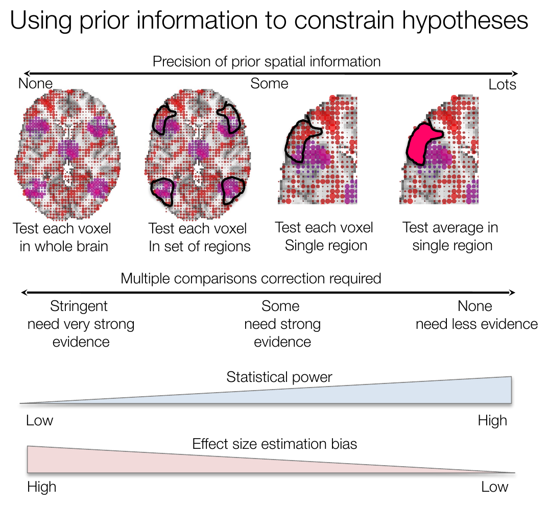
Using prior information to constrain hypotheses. Moving from whole-brain voxel-wise testing (left) toward averaging within a single a priori region (right) reduces the multiple comparisons correction required, increases statistical power, and decreases effect-size estimation bias — but demands increasingly precise prior spatial knowledge. (Figure 6.5 from the book. © the authors and MIT Press; reproduced with permission — not covered by this site’s CC-BY license.)
Finally, the validity of any statistical map rests on assumptions. Standard statistical ones include IID errors (noise is independent across observations, independent of the task, and drawn from one population), normality and equal variance, and correct model specification (event timing, duration, and hemodynamics are modeled correctly, and responses are linear in the predictors). Deeper assumptions concern how the brain implements task effects: that effects are localizable to discrete regions (questionable for diffuse neuromodulatory systems like dopamine), that background processes can be “subtracted off” (pure insertion — violated whenever adding a task changes what other processes do), that single voxels are meaningful independent units (whereas much evidence points to distributed population codes spanning many voxels), and that the largest, most reliable hemodynamic responses mark the most important areas. All of these are violated in some cases — so P values deserve a grain of salt, and true understanding comes from replication and converging evidence across methods. Still, as George Box put it, “all models are wrong, but some are useful”: statistical mapping, however imperfect, yields a great deal of reliable, reproducible information about the physiological basis of mental processes.
Hands-on tutorial
The best way to understand what a brain map is — and is not — is to build one from data where you know the ground truth. Here we run the complete brain-mapping loop in miniature: simulate a two-condition experiment at many “voxels” on a 2-D grid, compute each subject’s [A − B] difference image, test the group effect at every voxel, threshold, and visualize the map. Because we planted the true signal ourselves, we can see exactly which surviving blobs are real and which are noise.
Step 1 — Simulate the experiment and test every voxel. True signal lives in two circular “regions”; every subject’s difference image is that signal plus noise. A one-sample t-test across subjects at each voxel gives the statistical map.
% Requires only base MATLAB + Statistics Toolbox
rng(6);                                % fix the random seed for reproducible results
nx = 40; ny = 40;                      % nx, ny = grid size: a 40 x 40 voxel "slice"
n_sub = 24;                            % n_sub = number of participants

[xx, yy] = meshgrid(1:nx, 1:ny);       % voxel coordinate grids
truth = ((xx-12).^2 + (yy-12).^2 < 25) | ((xx-28).^2 + (yy-25).^2 < 25);   % two circular regions
true_effect = 1.0 * truth;             % true [A - B] effect: 1 inside the regions, 0 elsewhere

% Each subject's [A - B] difference image = true effect + noise (SD = 1)
diff_imgs = repmat(true_effect, 1, 1, n_sub) + randn(ny, nx, n_sub);

% One-sample t-test across subjects, separately at every voxel
[~, p_map, ~, stats] = ttest(diff_imgs, 0, 'dim', 3);
t_map = stats.tstat;

fprintf('Tested %d voxels; %d truly active\n', numel(t_map), sum(truth(:)));
fprintf('Largest t = %.1f; smallest p = %.1e\n', max(t_map(:)), min(p_map(:)));
import numpy as np
from scipy import stats
rng = np.random.default_rng(6) # fix the random seed for reproducible results
nx = ny = 40 # nx, ny = grid size: a 40 x 40 voxel "slice"
n_sub = 24 # n_sub = number of participants
xx, yy = np.meshgrid(np.arange(nx), np.arange(ny)) # voxel coordinate grids
truth = ((xx-12)**2 + (yy-12)**2 < 25) | ((xx-28)**2 + (yy-25)**2 < 25) # two circular regions
true_effect = 1.0 * truth # true [A - B] effect: 1 inside the regions, 0 elsewhere
# Each subject's [A - B] difference image = true effect + noise (SD = 1)
diff_imgs = true_effect + rng.standard_normal((n_sub, ny, nx))
# One-sample t-test across subjects, separately at every voxel
t_map, p_map = stats.ttest_1samp(diff_imgs, 0, axis=0)
print(f"Tested {t_map.size} voxels; {truth.sum()} truly active")
print(f"Largest t = {t_map.max():.1f}; smallest p = {p_map.min():.1e}")Example output:
Tested 1600 voxels; 138 truly active
Largest t = 8.5; smallest p = 1.5e-08
Step 2 — Threshold and visualize the map. Compare no correction against Bonferroni correction for the 1,600 tests, and see the tradeoff from Figure 6.4 come alive: lenient thresholds sprinkle false positives across the map, stringent ones miss parts of the true regions.
alpha = 0.05;                          % alpha = acceptable false positive rate per test
n_vox = nx * ny;                       % n_vox = number of tests in the family (1,600)
sig_unc  = p_map < alpha;              % uncorrected: expect ~5% of null voxels to pass
sig_bonf = p_map < alpha / n_vox;      % Bonferroni: controls family-wise error rate

figure;
subplot(1, 3, 1); imagesc(t_map); axis image off; title('t map');
subplot(1, 3, 2); imagesc(t_map .* sig_unc);  axis image off; title('p < .05 uncorrected');
subplot(1, 3, 3); imagesc(t_map .* sig_bonf); axis image off; title('Bonferroni corrected');
colormap hot;
import matplotlib.pyplot as plt
alpha = 0.05 # alpha = acceptable false positive rate per test
n_vox = nx * ny # n_vox = number of tests in the family (1,600)
sig_unc = p_map < alpha # uncorrected: expect ~5% of null voxels to pass
sig_bonf = p_map < alpha / n_vox # Bonferroni: controls family-wise error rate
fig, axes = plt.subplots(1, 3, figsize=(10, 3.5))
for ax, img, title in zip(axes, [t_map, t_map * sig_unc, t_map * sig_bonf],
["t map", "p < .05 uncorrected", "Bonferroni corrected"]):
ax.imshow(img, cmap="hot"); ax.set_title(title); ax.axis("off")Example output:
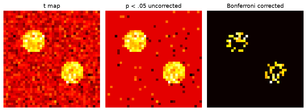
The two true regions stand out in all three panels — but the uncorrected map (209 significant voxels) is speckled with false positives across the “brain,” while Bonferroni correction (54 voxels) keeps essentially only true signal at the cost of missing the regions’ edges.
The full labs carry the loop further: building the single-subject map from trial-level data first, controlling the false discovery rate as a middle ground, counting true and false positives against the known truth, demonstrating how selecting significant voxels inflates effect-size estimates, and testing an a priori ROI — correctly placed and slightly misplaced — to feel both ends of the continuum in Figure 6.5. The MATLAB lab closes with the same voxel-wise t-test run on a real dataset using CANlab tools.
Open the full Python lab notebook → or download the MATLAB live script, which mirrors it and adds a real-data voxel-wise t-test with CANlab tools.


Thought questions
A newspaper prints a thresholded group map with the caption “the brain’s empathy center lights up.” Using the distinction between a statistical construction and a direct measurement, write a more accurate one-sentence caption — and identify at least two inferential steps the original caption glosses over.
A clinical team wants to use a single-subject map to argue in court that a defendant’s brain “functions abnormally.” What would need to be true — about the map’s construction, its comparison population, and the assumptions of Section 6.3 — for that claim to be sound? Which link in the chain seems weakest to you?
Suppose dopamine-driven effects of reward are genuinely diffuse, elevating activity slightly across most of the brain. Walk through what a voxel-wise map of [Reward − Neutral] with stringent FWER correction would show, and explain how a reader could be systematically misled about the neural architecture of reward.
Your colleague reports an a priori amygdala ROI analysis that “confirmed” their hypothesis, but you learn they also examined five other ROIs and several alternative preprocessing pipelines. Using the concepts of multiple comparisons, P-hacking, and HARKing, explain precisely what has gone wrong with the reported P value — even though every individual analysis was performed correctly.
Thresholded maps show only voxels with strong evidence, yet the chapter argues that surviving voxels’ effect sizes are systematically overestimated while non-significant voxels may still contain signal. If you could redesign the conventions for displaying brain maps in papers, what would you change, and what new misinterpretations might your conventions invite?
Quiz yourself
Q1. What do the colored regions in a typical published brain map represent?
Answer: The results of statistical hypothesis tests performed at each voxel — regions where a test statistic (e.g., a t value) exceeded a significance threshold, color-coded by the strength of the evidence. They are statistical constructions, not direct pictures of brain activity.
Q2. What is the key difference between a single-subject map and a group-level map, and which supports population inference?
Answer: A single-subject map tests effects within one person’s data (e.g., [Task − Control] across that person’s time series); a group-level map combines per-subject difference images and tests whether the effect is consistent across people, treating participants as a random effect. Only group-level maps support inferences about how brains work in general across the population.
Q3. In the brain-mapping generative model, what two components combine to produce the observed data, and what does the t-statistic measure?
Answer: True task-induced signal and stochastic noise combine additively; only their mixture is observed. The t-statistic is the estimated effect magnitude divided by its standard error — the evidence that a voxel’s true effect is non-zero, given how much estimates vary by chance.
Q4. With 30 participants, a voxel shows t = 1.7, corresponding to P = 0.10. What exactly does that P value mean, and what should we conclude at alpha = 0.05?
Answer: If the true effect were exactly zero, there would be a 10% chance of observing a t value of 1.7 or more extreme. Since 0.10 > 0.05, the voxel is called non-significant — but this does not prove the effect is absent; the evidence is simply insufficient.
Q5. What do family-wise error rate (FWER) and false discovery rate (FDR) corrections each control?
Answer: FWER correction controls the probability of observing any false positive voxel across the entire family of tests. FDR correction controls the expected proportion of significant voxels that are false positives. FDR is less stringent and typically yields more significant voxels than FWER control.
Q6. A voxel survives stringent correction in a group map. What claim does this license, and what claim does it not license?
Answer: It licenses the claim that the voxel has some non-zero effect in the population. It does not tell you the effect is large or meaningful — and because significant voxels are selected partly for favorable noise, their estimated effect sizes are biased upward.
Q7. What are the main advantages and risks at each end of the whole-brain versus single-ROI continuum?
Answer: Whole-brain voxel-wise mapping needs no precise prior hypothesis and can reveal unexpected effects, but requires stringent multiple comparisons correction, which lowers power and inflates apparent effect sizes in surviving voxels. A single a priori ROI maximizes power and avoids selection bias, but only if the hypothesis is correct — a slightly misplaced ROI can miss a real effect entirely.
Q8. Name the “pure insertion” assumption and give an example of how it can fail.
Answer: Pure insertion assumes that adding a task component changes only the process of interest, so background processes can be subtracted off in a [Task − Control] comparison. It fails whenever adding the new component alters the other computations being performed — for example, if adding a memory demand changes how a region processes the visual stimuli present in both conditions.
 The book: Elements of Functional Magnetic Resonance Imaging — Wager & Lindquist, MIT Press