Forward and Reverse Inference
Run this code: ⚡ In-browser lab · Colab · MATLAB Online
Overview
Brain mapping is well suited to one kind of question and poorly suited to another. When we induce a psychological state — pain, fear, punishment motivation — and ask which regions respond, we are making a forward inference: we learn about the probability of brain activity given a psychological state, written . In the language of diagnostic testing, this is the sensitivity (or hit rate) of the brain measure. Standard brain maps are precisely this: maps of forward inference. The stronger the statistical effect, the more likely a region “lights up” when the state is present.
Often, though, what we really want is the opposite direction. If the caudate nucleus is active, can we conclude that a person is experiencing punishment motivation? That is a reverse inference — the probability of a mental state given brain activity, — known in the diagnostic literature as the positive predictive value (PPV) of the test. If we could make such inferences reliably, we could “decode” mental states from brain activity: infer whether someone is in pain, engaging cognitive effort, or hiding information.
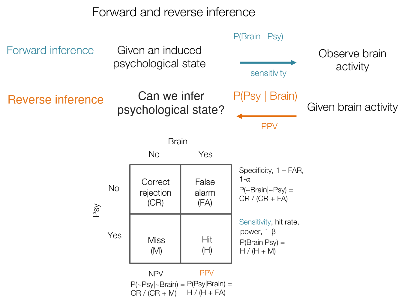
Forward and reverse inference applied to brain mapping, and their relationship with diagnostic testing measures. “Brain” refers to a brain measure being present (e.g., activation above threshold); “Psy” refers to an underlying psychological state being present. Sensitivity is ; specificity is ; PPV is . In the two-by-two table, is the empirical false-positive rate (1 − specificity), the miss rate (1 − sensitivity), FAR the false alarm rate, and NPV the negative predictive value. (Figure 7.1 from the book. © the authors and MIT Press; reproduced with permission — not covered by this site’s CC-BY license.)
The catch is that forward and reverse inference are not interchangeable. A region can respond reliably to a task without being informative about that task, because most brain structures respond to many things — there is a many-to-many mapping between psychological constructs and brain regions. The caudate is strongly activated by reward, cognitive control, motor behavior, and more; even 99% sensitivity to punishment decisions would not make caudate activation good evidence of punishment motivation. Treating it as such is the classical logical fallacy of affirming the consequent: if all dogs prefer ice cream over fruit, and Mary prefers ice cream, it does not follow that Mary is a dog. says nothing about until we consider .
Bayes’ rule makes the relationship exact:
P(Psy | Brain) — reverse inference (PPV) · P(Brain | Psy) — forward inference (sensitivity) · P(Psy) — base rate of the mental state · P(Brain) — overall probability of the brain response, across all states
where is the reverse inference (the PPV), the forward inference (sensitivity), the base rate of the mental state, and the overall probability of observing the brain response across all states, present or absent.
Expanding the denominator over the state being present or absent gives the PPV as a function of three quantities — sensitivity, specificity (, i.e., how rarely the region activates in the absence of the state), and the base rate (the proportion of time the state occurs at all):
PPV — positive predictive value, P(Psy | Brain) · Sens — sensitivity, P(Brain | Psy) · Spec — specificity, P(~Brain | ~Psy) · P(Psy) — base rate of the state · P(~Psy) — probability the state is absent, 1 − P(Psy)
where is the positive predictive value , the sensitivity , the specificity , the base rate of the state, and the probability that the state is absent.
Plugging in numbers is sobering. Suppose the caudate responds to punishment motivation with 90% sensitivity and 80% specificity, and people experience that state 10% of the time (probably generous). Observing caudate activity then implies punishment motivation with probability of only 33% — nowhere near the 90% sensitivity. Raising sensitivity to a perfect 100% barely helps (PPV = 36%). But drop the base rate to 1% and the PPV collapses to 4%. PPV is driven by specificity and base rate, not sensitivity — and standard brain maps measure only sensitivity. The same arithmetic bedevils medical screening: mammography has roughly 90% sensitivity and 80–99% specificity, but with a ~1.5% ten-year base rate of breast cancer in 40–50-year-old women, the PPV of a positive screen is only about 6% in the U.S. (at 80% specificity) versus about 40% in Denmark (at 98% specificity).
Valid reverse inference is possible — it just requires evaluating specificity against the alternatives, not merely showing that a region activates. That means testing a brain measure across many confusable states: task conditions, mental constructs, and behaviors that could produce the same activation. Meta-analytic databases such as Neurosynth aggregate results from thousands of studies, allowing brain patterns to be compared against hundreds of psychological terms and supporting empirically grounded reverse-inference maps. Large multi-task datasets and naturalistic paradigms push in the same direction. And because averaging over a whole structure (the hippocampus, say) mixes many circuits with many functions, multivariate pattern analysis — training algorithms to find the fine-grained features that best discriminate a state from thousands of alternatives — is a particularly promising route. Properly validated, such brain measures could let us assess pain, emotion, and cognition in people who cannot report them, and reveal which brain systems treatments actually act on.
Hands-on tutorial
In this tutorial you will implement Bayes’ rule as a reverse-inference calculator, reproduce the chapter’s caudate example, and see quantitatively how selective a region must be — and how common a mental state must be — before its activation supports a confident reverse inference. The full labs extend this to a simulated likelihood-ratio “reverse inference map” in the spirit of Neurosynth.
Step 1 — Compute PPV from sensitivity, specificity, and base rate. We implement the PPV equation and evaluate the chapter’s toy example: 90% sensitivity, 80% specificity, 10% base rate.
% PPV from sensitivity, specificity, and base rate (Bayes' rule)
ppv = @(sens, spec, br) (sens .* br) ./ ...
      (sens .* br + (1 - spec) .* (1 - br));

% Chapter example: caudate and punishment motivation
fprintf('Sens 0.90, Spec 0.80, BR 0.10 -> PPV = %.2f\n', ppv(.90, .80, .10));  % chapter values: sens, spec, base rate
fprintf('Sens 1.00 (perfect!)         -> PPV = %.2f\n', ppv(1.0, .80, .10));   % perfect sensitivity, same spec and base rate
fprintf('Base rate 0.01               -> PPV = %.2f\n', ppv(.90, .80, .01));   % rare state: base rate drops to 1%
import numpy as np
def ppv(sens, spec, base_rate):
"""PPV from sensitivity, specificity, and base rate (Bayes' rule)."""
sens, spec, br = np.asarray(sens), np.asarray(spec), np.asarray(base_rate)
return sens * br / (sens * br + (1 - spec) * (1 - br))
# Chapter example: caudate and punishment motivation
print(f"Sens 0.90, Spec 0.80, BR 0.10 -> PPV = {ppv(.90, .80, .10):.2f}") # chapter values: sens, spec, base rate
print(f"Sens 1.00 (perfect!) -> PPV = {ppv(1.0, .80, .10):.2f}") # perfect sensitivity, same spec and base rate
print(f"Base rate 0.01 -> PPV = {ppv(.90, .80, .01):.2f}") # rare state: base rate drops to 1%Example output:
Sens 0.90, Spec 0.80, BR 0.10 -> PPV = 0.33
Sens 1.00 (perfect!)          -> PPV = 0.36
Base rate 0.01                -> PPV = 0.04
You should get PPV = 0.33, 0.36, and 0.04 — matching the chapter. Perfect sensitivity buys almost nothing; a rarer state destroys the inference.
Step 2 — How selective must a region be? We sweep specificity from 0.5 to 1 at several base rates and ask: how specific must activation be for a confident (PPV ≥ 0.9) reverse inference?
spec = linspace(.5, .999, 200);   % spec = specificity grid, chance (0.5) to near-perfect
base_rates = [.5 .1 .01];         % base_rates = P(Psy): common, uncommon, rare

figure; hold on;
for br = base_rates
    plot(spec, ppv(.90, spec, br), 'LineWidth', 2, ...
        'DisplayName', sprintf('base rate = %g', br));
end
yline(.9, '--', 'PPV = 0.9'); xlabel('Specificity'); ylabel('PPV');
title('Reverse inference needs specificity AND a decent base rate');
legend('Location', 'northwest');
import matplotlib.pyplot as plt
spec = np.linspace(0.5, 0.999, 200) # spec = specificity grid, chance (0.5) to near-perfect
fig, ax = plt.subplots(figsize=(6, 4))
for br in [0.5, 0.1, 0.01]: # br = base rate P(Psy): common, uncommon, rare
ax.plot(spec, ppv(0.90, spec, br), lw=2, label=f"base rate = {br}")
ax.axhline(0.9, ls="--", color="gray")
ax.set(xlabel="Specificity", ylabel="PPV = P(Psy | Brain)",
title="Reverse inference needs specificity AND a decent base rate")
ax.legend()Example output:
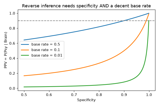
PPV rises with specificity, but at low base rates even near-perfect specificity barely supports a confident reverse inference.
At a 10% base rate, even 99% specificity yields a PPV of about 0.91 — barely clearing the bar — and at a 1% base rate no realistic specificity suffices for a single region. This is why open-ended tests across many alternative states, and multivariate patterns tuned for discrimination, are central to modern reverse inference.
Open the full Python lab notebook → or download the MATLAB live script, which mirrors it and adds an optional CANlab/Neurosynth similarity example.


Thought questions
A widely cited study reports that the insula activates in 30% of all published fMRI studies, spanning pain, emotion, interoception, salience, and language. A newspaper headline announces that a defendant’s insula activation during testimony “reveals he felt genuine remorse.” Deconstruct this claim using sensitivity, specificity, and base rate — which quantity does each piece of evidence in the study actually speak to?
Neurosynth computes both “forward inference” maps () and “reverse inference” (association) maps that account for how often activation appears across all other terms. Why can these two maps look dramatically different for the same term (e.g., “pain”), and which regions would you expect to survive in the reverse map but not dominate the forward map?
The base rate is straightforward for a disease (prevalence), but what does it even mean for a mental state like “punishment motivation” occurring in daily life versus within a specific experimental task context? How does constraining the context (e.g., “given the participant is doing one of these 10 tasks”) change the Bayesian calculation, and is that constrained inference still useful?
Multivariate predictive models are said to enable valid reverse inference because they are optimized and tested for discrimination among alternatives. What would a convincing specificity evaluation for a “pain signature” look like — which alternative conditions must be tested, and why is averaging activity over a whole anatomical region unlikely to achieve the same specificity?
Screening programs (e.g., mammography under age 40) are sometimes abandoned not because the test is insensitive but because the PPV is too low. Propose an fMRI-based “biomarker” use case, estimate plausible sensitivity, specificity, and base rate, and argue whether deployment would be justified.
Quiz yourself
Q1. Define forward inference and reverse inference as conditional probabilities.
Answer: Forward inference is the probability of brain activity given a psychological state, . Reverse inference is the probability of the psychological state given brain activity, .
Q2. Which diagnostic-testing quantities correspond to forward and reverse inference?
Answer: Forward inference corresponds to sensitivity (hit rate, recall); reverse inference corresponds to the positive predictive value (PPV) of the test.
Q3. What is specificity, and how is it written in probability notation?
Answer: Specificity is the probability that the brain measure does not respond when the state is absent: , which equals 1 minus the false alarm rate.
Q4. Write Bayes’ rule relating to .
Answer: — sensitivity times the base rate of the state, divided by the overall probability of observing the brain measure across all states.
Q5. In the chapter’s caudate example (90% sensitivity, 80% specificity, 10% base rate), roughly what is the PPV, and what happens when sensitivity rises to 100%?
Answer: The PPV is only about 33%. Raising sensitivity to 100% increases it only to about 36% — PPV is driven by specificity and base rate, not sensitivity.
Q6. What logical fallacy is committed when strong forward inference is used to claim reverse inference, and what is the ice-cream illustration?
Answer: Affirming the consequent. Even if every dog prefers ice cream over fruit (), someone who prefers ice cream is not therefore a dog — the inference ignores , i.e., how often the observation occurs without the state.
Q7. Why can’t averaging activity across an entire structure like the hippocampus establish that its activation implies memory?
Answer: The hippocampus (like most structures) contains many circuits participating in many mental functions, so its average activity is not specific to memory. Establishing reverse inference requires showing specificity against alternative processes — for which fine-grained multivariate patterns, tested across many alternatives, are more promising.
Q8. Name two developments that make open-ended tests of specificity across many mental states feasible.
Answer: Large meta-analytic databases aggregating thousands of studies (e.g., Neurosynth), large multi-task datasets, and naturalistic experiments exposing participants to thousands of images and concepts — any two of these.
 The book: Elements of Functional Magnetic Resonance Imaging — Wager & Lindquist, MIT Press