Chapter 7 Lab — Forward and Reverse Inference (Python) - Elements of fMRI Analysis

Standard brain maps tell us the probability of activation given a psychological state — forward inference, or sensitivity. What we usually want is the probability of the state given activation — reverse inference, or positive predictive value (PPV). In this lab you will implement Bayes’ rule as a reverse-inference calculator, verify it with a Monte Carlo simulation, explore how PPV depends on specificity and base rate, and build a toy “reverse inference map” that shows why forward-inference maps and reverse-inference maps of the same state can look very different.

How to run this notebook: it runs in the browser (Pyodide), on Google Colab, or locally — it uses only numpy, pandas, and matplotlib, with simulated data. Companion reading: the Chapter 7 tutorial page.

▶ This notebook is interactive. Click the ⏻ power icon at the top right of this page to run it in your browser — no installation needed (the kernel takes ~30–60 s to start the first time). Then run cells top to bottom, starting with the first code cell below: later cells depend on the imports and variables defined earlier, and will error if you skip ahead.

import numpy as np
import pandas as pd
import matplotlib.pyplot as plt

rng = np.random.default_rng(7)      # seed = 7 -> reproducible simulated data
plt.rcParams["figure.dpi"] = 100    # inline figure resolution

1. Bayes’ rule as a reverse-inference calculator¶

Forward inference is $P(\text{Brain} \mid \text{Psy})$ — the sensitivity of a brain measure to a psychological state. Reverse inference is $P(\text{Psy} \mid \text{Brain})$ — the PPV. Bayes’ rule connects them:

P(\text{Psy} \mid \text{Brain}) = \frac{P(\text{Brain} \mid \text{Psy})\,P(\text{Psy})}{P(\text{Brain})} = \frac{\text{Sens} \times \text{BR}}{\text{Sens} \times \text{BR} + (1-\text{Spec})(1-\text{BR})}

(1)

P(Psy | Brain) — reverse inference (PPV) · P(Brain | Psy) — forward inference · Sens — sensitivity · Spec — specificity, P(~Brain | ~Psy) · BR — base rate P(Psy)

where $P(\text{Psy} \mid \text{Brain})$ is the reverse inference (the PPV), $P(\text{Brain} \mid \text{Psy})$ the forward inference, $\text{Sens}$ the sensitivity, $\text{Spec}$ the specificity $P(\sim\text{Brain} \mid \sim\text{Psy})$ , and $\text{BR}$ the base rate $P(\text{Psy})$ of the state.

Let’s implement this and reproduce the chapter’s caudate / punishment-motivation example.

def ppv(sens, spec, base_rate):
    """Positive predictive value P(Psy | Brain) via Bayes' rule.

    sens      : P(Brain | Psy)        -- sensitivity (forward inference)
    spec      : P(~Brain | ~Psy)      -- specificity
    base_rate : P(Psy)                -- prior probability of the state
    """
    sens, spec, br = np.asarray(sens), np.asarray(spec), np.asarray(base_rate)
    return sens * br / (sens * br + (1 - spec) * (1 - br))


# The chapter's toy example: caudate activation and punishment motivation
scenarios = pd.DataFrame(
    [
        ["Chapter example",            0.90, 0.80, 0.10],
        ["Perfect sensitivity",        1.00, 0.80, 0.10],
        ["Rare state (1% base rate)",  0.90, 0.80, 0.01],
        ["Highly specific region",     0.90, 0.99, 0.10],
        ["Specific AND common state",  0.90, 0.99, 0.50],
    ],
    columns=["scenario", "sensitivity", "specificity", "base_rate"],
)
scenarios["PPV"] = ppv(scenarios.sensitivity, scenarios.specificity,
                       scenarios.base_rate).round(3)
scenarios

The first three rows reproduce the chapter’s numbers: PPV = 0.33 despite 90% sensitivity; perfect sensitivity barely helps (0.36); a 1% base rate collapses the PPV to 0.04. Only when the region is highly specific and the state is reasonably common does activation become strong evidence for the state.

Monte Carlo check¶

Bayes’ rule is exact, but it is worth seeing it emerge from raw counts. Simulate 200,000 “moments of mental life”: in each moment the state is present with probability equal to the base rate, and the region activates with probability = sensitivity (state present) or 1 − specificity (state absent). Then simply count: among the moments where the region was active, in what fraction was the state actually present?

n = 200_000                                    # number of simulated "moments of mental life"
sens, spec, br = 0.90, 0.80, 0.10              # sensitivity, specificity, base rate (chapter example)

psy = rng.random(n) < br                       # is the state present?
p_act = np.where(psy, sens, 1 - spec)          # P(activation) this moment
brain = rng.random(n) < p_act                  # does the region activate?

counts = pd.crosstab(pd.Series(psy, name="Psy"),
                     pd.Series(brain, name="Brain"))
print(counts, "\n")
print(f"Empirical P(Psy | Brain) = {psy[brain].mean():.3f}")
print(f"Analytic  PPV            = {ppv(sens, spec, br):.3f}")

Brain   False  True 
Psy                 
False  143961  36306
True     1989  17744 

Empirical P(Psy | Brain) = 0.328
Analytic  PPV            = 0.333

The empirical fraction matches Bayes’ rule. Notice why the PPV is low in the crosstab: the state is rare, so even a modest false-alarm rate (1 − specificity = 20%) applied to the huge number of state-absent moments produces far more false alarms than there are hits.

2. How selective must a region be?¶

Suppose we insist on a confident reverse inference — say PPV ≥ 0.9 (“if this region is active, I am ≥90% sure the state is present”). How specific must the region’s activation be? We sweep specificity at several base rates, holding sensitivity at 0.9.

spec_grid = np.linspace(0.5, 0.999, 300)   # specificity grid, chance (0.5) to near-perfect
base_rates = [0.5, 0.25, 0.10, 0.01]       # base rates P(Psy), common to rare

fig, ax = plt.subplots(figsize=(7, 4.5))
for br in base_rates:
    ax.plot(spec_grid, ppv(0.90, spec_grid, br), lw=2,
            label=f"base rate = {br}")
ax.axhline(0.9, color="gray", ls="--", lw=1)
ax.text(0.505, 0.915, "PPV = 0.9 (confident reverse inference)",
        color="gray", fontsize=9)
ax.set(xlabel="Specificity, P(~Brain | ~Psy)",
       ylabel="PPV = P(Psy | Brain)",
       title="PPV vs. specificity (sensitivity fixed at 0.90)")
ax.legend(loc="center left")
plt.tight_layout()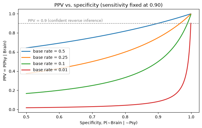

We can also solve the PPV equation for the required specificity. Setting PPV = $p$ (the target PPV we insist on) and rearranging:

\text{Spec}_{\text{required}} = 1 - \frac{\text{Sens} \times \text{BR} \times (1-p)}{p\,(1-\text{BR})}

(2)

Spec_required — specificity needed to reach the target PPV · Sens — sensitivity · BR — base rate P(Psy) · p — target PPV

where $\text{Spec}_{\text{required}}$ is the specificity needed to reach the target PPV, $\text{Sens}$ the sensitivity, $\text{BR}$ the base rate $P(\text{Psy})$ , and $p$ the target PPV.

def required_specificity(sens, base_rate, target_ppv):
    """Specificity needed to reach target_ppv (may exceed 1 = impossible)."""
    sens, br, p = np.asarray(sens), np.asarray(base_rate), target_ppv
    return 1 - sens * br * (1 - p) / (p * (1 - br))


br_grid = np.array([0.50, 0.25, 0.10, 0.05, 0.01, 0.001])   # base rates, common (50%) to very rare (0.1%)
req = pd.DataFrame({
    "base_rate": br_grid,
    "required_spec_PPV_0.80": required_specificity(0.9, br_grid, 0.80).round(4),
    "required_spec_PPV_0.90": required_specificity(0.9, br_grid, 0.90).round(4),
    "required_spec_PPV_0.95": required_specificity(0.9, br_grid, 0.95).round(4),
})
req

At a 50% base rate, ~89% specificity suffices for PPV = 0.9. At a 10% base rate you already need 99% specificity. At a 1% base rate you need ~99.9% — the region would have to activate almost never in the absence of the state. For rare states, no single anatomical region is plausibly that selective: this is why reverse inference from “area X lit up” fails, and why the field has turned to fine-grained multivariate patterns explicitly optimized and tested for specificity.

3. Base rates rule: the screening problem¶

The same arithmetic governs medical screening. Mammography has ~90% sensitivity and 80–99% specificity depending on setting, yet for 40–50-year-old women (10-year base rate of breast cancer ≈ 1.5%) a positive screen implies cancer with probability of only ~6% at 80% specificity — or ~40% at 98% specificity. Let’s plot PPV as a function of base rate for these two specificities.

br_grid = np.logspace(-3, 0, 400)            # base rates from 0.1% to 100%

fig, ax = plt.subplots(figsize=(7, 4.5))
for spec, label in [(0.80, "specificity = 0.80 (US mammography)"),
                    (0.98, "specificity = 0.98 (Denmark)")]:
    ax.semilogx(br_grid, ppv(0.90, spec, br_grid), lw=2, label=label)

br_mammo = 0.0147   # 10-year breast cancer base rate, women age 40-50 (ACS 2017-2018)
for spec, c in [(0.80, "C0"), (0.98, "C1")]:
    ax.plot(br_mammo, ppv(0.90, spec, br_mammo), "o", color=c, ms=8)
ax.axvline(br_mammo, color="gray", ls=":", lw=1)
ax.text(br_mammo * 1.15, 0.62, "10-yr breast cancer\nbase rate, age 40-50",
        fontsize=9, color="gray")
ax.set(xlabel="Base rate P(Psy)  [log scale]", ylabel="PPV",
       title="PPV vs. base rate (sensitivity = 0.90)")
ax.legend(loc="upper left")
plt.tight_layout()

print(f"PPV at base rate 1.47%: spec 0.80 -> {ppv(.9, .80, br_mammo):.3f}, "
      f"spec 0.98 -> {ppv(.9, .98, br_mammo):.3f}")

PPV at base rate 1.47%: spec 0.80 -> 0.063, spec 0.98 -> 0.402

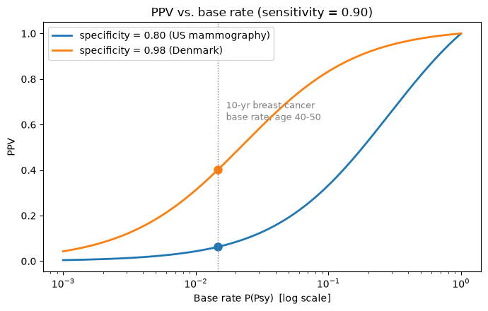
Both curves have high sensitivity, yet at low base rates the PPV differs by nearly an order of magnitude depending on specificity — and both are far below what the sensitivity alone suggests. Translational neuroimaging faces exactly this issue: case–control studies of depression, dementia, or chronic pain rarely assess the base rates of the disorders in the populations where a biomarker would actually be deployed.

4. A toy reverse-inference map (the Neurosynth idea)¶

Meta-analytic databases like Neurosynth make this concrete for whole brain maps. A forward-inference map shows $P(\text{activation} \mid \text{term})$ — how consistently a voxel activates in studies about, say, pain. A reverse-inference (association) map instead asks how diagnostic activation is of the term, accounting for how often the voxel activates across all other kinds of studies.

We simulate a small 2D “brain” with two active regions:

Region S (selective): activates strongly for our target state, rarely otherwise.
Region G (general): activates strongly for the target state and for many other states — like the “salience network” regions that appear in a huge fraction of all fMRI studies.

Each voxel has a sensitivity $P(\text{act} \mid \text{Psy})$ and a false-alarm rate $P(\text{act} \mid \sim\text{Psy})$ . From these we compute the likelihood ratio $LR = \frac{P(\text{act} \mid \text{Psy})}{P(\text{act} \mid \sim\text{Psy})}$ and the posterior map $P(\text{Psy} \mid \text{act})$ at a given base rate.

def gauss2d(shape, center, width):
    yy, xx = np.mgrid[0:shape[0], 0:shape[1]]
    return np.exp(-((xx - center[1]) ** 2 + (yy - center[0]) ** 2)
                  / (2 * width ** 2))

shape = (48, 64)      # toy "brain": 48 x 64 voxels

# P(act | Psy): BOTH regions respond strongly to the target state
sens_map = 0.05 + 0.85 * (gauss2d(shape, (16, 18), 5)      # Region S
                          + gauss2d(shape, (30, 46), 6))   # Region G
sens_map = np.clip(sens_map, 0, 0.95)                      # cap sensitivity at 95%

# P(act | ~Psy): only Region G also responds to many OTHER states
fa_map = 0.05 + 0.65 * gauss2d(shape, (30, 46), 6)
fa_map = np.clip(fa_map, 0, 0.90)                          # cap false-alarm rate at 90%

base_rate = 0.10      # prior probability P(Psy) of the state
lr_map = sens_map / fa_map                                  # likelihood ratio
posterior_map = ppv(sens_map, 1 - fa_map, base_rate)        # P(Psy | act)

fig, axes = plt.subplots(1, 3, figsize=(13, 3.6))
for ax, img, title, cmap in [
        (axes[0], sens_map, "Forward map: P(act | Psy)\n(what brain maps show)", "hot"),
        (axes[1], lr_map, "Likelihood ratio:\nP(act | Psy) / P(act | ~Psy)", "viridis"),
        (axes[2], posterior_map, f"Reverse map: P(Psy | act)\nbase rate = {base_rate}", "hot")]:
    im = ax.imshow(img, cmap=cmap)
    ax.set(title=title, xticks=[], yticks=[])
    fig.colorbar(im, ax=ax, shrink=0.85)
axes[0].annotate("S", (18, 16), color="cyan", fontsize=14, weight="bold")
axes[0].annotate("G", (46, 30), color="cyan", fontsize=14, weight="bold")
plt.tight_layout()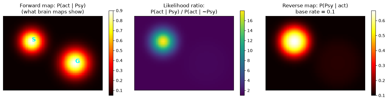

In the forward map (left), regions S and G look almost identical — both are “reliably activated by the task,” and a standard group analysis would report both. But the likelihood ratio and the posterior reverse-inference map (right) tell a different story: only the selective region S carries real evidence about the state. Region G, which responds to nearly everything, is almost uninformative — its posterior barely exceeds the base rate.

def summarize(name, yx):
    s, f = sens_map[yx], fa_map[yx]
    print(f"Region {name}: sens = {s:.2f}, P(act|~Psy) = {f:.2f}, "
          f"LR = {s / f:5.1f}, P(Psy|act) = {ppv(s, 1 - f, base_rate):.2f}")

summarize("S (selective)", (16, 18))
summarize("G (general)  ", (30, 46))
print(f"\nPrior P(Psy) = {base_rate:.2f}")

Region S (selective): sens = 0.90, P(act|~Psy) = 0.05, LR =  18.0, P(Psy|act) = 0.67
Region G (general)  : sens = 0.90, P(act|~Psy) = 0.70, LR =   1.3, P(Psy|act) = 0.13

Prior P(Psy) = 0.10

Activation in region S raises the probability of the state from the 10% prior to roughly 65%; activation in region G leaves it near 12%. Same forward inference, radically different reverse inference — the entire difference lies in $P(\text{act} \mid \sim\text{Psy})$ , which standard brain maps never measure.

Wrap-up¶

Forward inference (sensitivity, $P(\text{Brain} \mid \text{Psy})$ ) is what standard brain maps deliver; reverse inference (PPV, $P(\text{Psy} \mid \text{Brain})$ ) is what mind-reading claims require.
Bayes’ rule shows PPV depends strongly on specificity and base rate, and only weakly on sensitivity.
For rare states, even extremely specific regions yield weak reverse inferences — and required specificity grows out of reach as base rate falls.
Valid reverse inference requires measuring $P(\text{act} \mid \sim\text{Psy})$ across many confusable alternatives — the logic behind Neurosynth’s association maps and specificity-tested multivariate signatures.

Next: Chapter 8 examines which inferences from brain maps are valid and which are not.