Valid and Invalid Inferences
Run this code: ⚡ In-browser lab · Colab · MATLAB Online
Overview
The basic brain mapping procedure behind most published neuroimaging findings performs a significance test at every voxel and marks the survivors as “activated.” As Chapter 7 explained, this supports forward inferences about the presence of some non-zero effect under an experimental manipulation. But the alternative hypothesis is vague — merely “not zero” — and it is surprising how many natural-seeming conclusions a thresholded map does not license. Forward inference maps are not very informative about (a) the spatial location of activity, (b) how large or meaningful effects are, (c) the overall pattern of active and inactive voxels, or (d) the overlap in neural processes across tasks. This chapter is about why — and the best way to internalize the lessons is to watch each failure happen in data you simulated yourself, which is exactly what the labs below do.
Spatial location. Perhaps the most prevalent misconception is that brain maps tell us where activity occurs. A map estimates the strength of evidence for a non-zero effect at each voxel, which creates an illusion of localization — but standard procedures provide no P values or confidence intervals on the location or boundaries of activation, because they do not model spatial variability across individuals and studies. That variability is substantial: point-spread blurring, draining-vein and inflow artifacts, registration error, scanner-specific distortions, and true individual differences in functional anatomy all displace the apparent location of effects, and reported peak coordinates — however precise their millimeters look — come from ad hoc peak-finding algorithms that are sensitive to noise. Across studies, peak locations for the same process can wander by roughly ±1–1.5 cm. Inferring where activity is, or whether two tasks activate reliably different places, requires explicit spatial statistics, such as confidence ellipsoids on peak locations across studies.
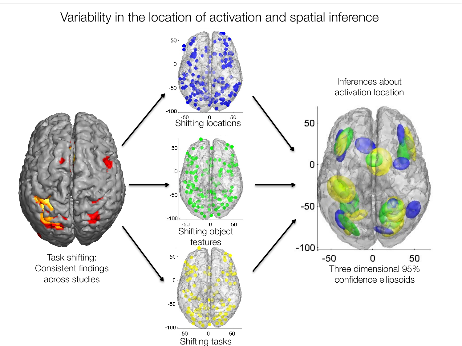
Variability in activation location across studies. Left: regions consistently activated across task-switching studies. Center: peak coordinates from individual studies for three types of attention shifting — the scatter is striking. Right: 3-D 95% spatial confidence ellipsoids for each shifting type; only where ellipsoids are separable can one infer that the types activate reliably different locations. (Figure 8.1 from the book. © the authors and MIT Press; reproduced with permission — not covered by this site’s CC-BY license.)
Effect size. A finding’s practical and clinical significance depends on how large the effect is, not on how small its P value is. Effect sizes describe effect strength in sample-size-free statistical units: Cohen’s is a mean difference divided by its standard deviation, and Pearson’s (or ) is the proportion of variance explained. The two families interconvert, and both link directly to test statistics — for a one-sample comparison across participants (where is the number of participants contributing one observation each),
t — one-sample t-statistic · d — Cohen’s d (mean difference ÷ its SD) · N — number of participants · r — Pearson correlation
where is the one-sample t-statistic, is Cohen’s d (the mean difference divided by its standard deviation), is the number of participants, and is the Pearson correlation being converted to an equivalent .
A tiny effect () can carry an astronomically small P value in a study of 100,000 people; sample size sharpens the precision of an effect size estimate but does not change its expected value. Interpretability matters too: a “moderate” effect of corresponds to only about 60% accuracy in classifying which condition an individual observation came from, and even a “large” yields only about 66% — a sobering calibration for anyone hoping to make inferences about individuals from group maps.
The selection bias problem. Here is the catch: standard brain maps cannot validly report effect sizes in significant regions at all. A whole-brain analysis runs hundreds of thousands of tests (~320,000 at 2-mm resolution), and thresholding selects the voxels where noise happened to push the estimate up. If every truly active voxel has , then with the estimates scatter roughly between and 0.88 — but significance at p < .001 requires an estimated , so every significant voxel overstates the true effect, some dramatically. Smaller samples and more stringent thresholds make the inflation worse, not better. Circular analysis — selecting voxels by one criterion (response to Task A) and then testing a non-independent effect (A − B) in them — is the same bias in another guise. This “winner’s curse” ignited the so-called voodoo correlations debate in social neuroscience, but it is a pervasive phenomenon: the golfer who reports only their 10 best holes looks like a pro, published drug trials outperform the ones left in the file drawer, and initially spectacular effects “decline” toward the true population value upon replication. The clean escapes are to test a single pre-defined region, or to build a predictive model that makes one prediction per participant and is evaluated on independent participants — in both cases, effect size estimates are unbiased.
Patterns of active and non-active voxels. Many psychological processes engage distributed brain systems, so we often want to infer the overall pattern of activation. Current multiple-comparisons practice is poorly suited to this: controlling the family-wise error rate demands thresholds so stringent that sensitivity collapses. With 30 participants and , power is about 80% for a single pre-specified region but plummets to roughly 2% at typical corrected voxel-wise thresholds — meaning a given truly active voxel would be detected in about one of every 50 studies. Researchers compensate by sacrificing spatial precision (cluster-extent thresholds, counting any activity “somewhere in dlPFC” as a replication), which quietly creates a false sense of replicability and undermines localization.
Overlap and dissociation across tasks. Double dissociations — damage 1 impairs Task A more than B, damage 2 impairs B more than A — have been a gold standard for separating mental processes, and imaging adopted the same logic by comparing activation maps. But with low power, any two thresholded maps will differ, even if the underlying process is identical, because which voxels survive is largely determined by noise. Interpretation then becomes a Rorschach test: theorists who expect overlap gaze at the shared voxels; theorists who expect separation point to the non-overlapping ones. Circularity compounds the damage — select a “Task A region” from the A map, extract responses to both tasks, and you will manufacture an impressive double dissociation from identical true effects. And even genuine voxel-level overlap is ambiguous: each voxel averages over ~5.5 million neurons, so two tasks can activate the same voxel via entirely different neural populations. A voxel that responds to pain is not a “pain voxel.” Valid dissociation inference requires independence — select regions in one sample, test the dissociation in another — and stronger claims require the predictive-modeling and pattern-based approaches covered later in the book.
Hands-on tutorial
These exercises reproduce several of the “statistical lies” simulations from the book’s companion code: you will generate data where you know the ground truth, run standard mapping analyses on it, and watch them mislead you. Two key demonstrations appear below in compact form; the full labs add null brain–behavior correlations, artifact “activations,” the independent-selection fix, and a PPV calculator.
Step 1 — The winner’s curse. Every voxel below has the same true effect, . We threshold at p < .001 and compare the average estimated effect size among significant voxels with the truth.
% Adapted from CANlab FMRI_simulations (github.com/canlab), statistical lies demos
rng(1);                                   % fixed seed for reproducibility
N = 30; n_vox = 20000; d_true = 0.5;      % N = participants; n_vox = voxels tested; d_true = true effect (Cohen's d) at EVERY voxel
data = randn(N, n_vox) + d_true;          % every voxel truly active, d = 0.5

d_hat = mean(data) ./ std(data);          % estimated effect size per voxel
t     = d_hat .* sqrt(N);                 % one-sample t-statistic
p     = 2 * tcdf(-abs(t), N - 1);         % two-tailed p value, N - 1 df

sig = p < .001;                           % "significant" voxels only (typical mapping threshold)
fprintf('True d = %.2f | mean estimated d: all voxels %.2f, significant voxels %.2f\n', ...
    d_true, mean(d_hat), mean(d_hat(sig)))
import numpy as np
from scipy import stats
rng = np.random.default_rng(1) # fixed seed for reproducibility
N, n_vox, d_true = 30, 20_000, 0.5 # N = participants; n_vox = voxels tested; d_true = true effect (Cohen's d) at EVERY voxel
data = rng.standard_normal((N, n_vox)) + d_true # every voxel truly active
d_hat = data.mean(0) / data.std(0, ddof=1) # estimated effect size per voxel
t = d_hat * np.sqrt(N) # one-sample t-statistic
p = 2 * stats.t.sf(np.abs(t), N - 1) # two-tailed p value, N - 1 df
sig = p < .001 # "significant" voxels only (typical mapping threshold)
print(f"True d = {d_true} | mean estimated d: all voxels {d_hat.mean():.2f}, "
f"significant voxels {d_hat[sig].mean():.2f}")Example output:
True d = 0.5 | mean estimated d: all voxels 0.51, significant voxels 0.80The significant voxels report — a 60% overstatement of a truth you built in yourself. No individual test did anything wrong; the bias lives entirely in the selection.
Step 2 — A false double dissociation. Tasks A and B have identical true effects at every voxel. We select an ROI from each task’s thresholded map and extract both tasks’ responses from both ROIs — the classic circular analysis.
% Adapted from lie9_false_double_dissociation.m (github.com/canlab FMRI_simulations)
rng(2);                                   % fixed seed for reproducibility
N = 20; n_vox = 5000; d_true = 0.3;       % N = participants; d_true = identical weak true effect for BOTH tasks, everywhere
taskA = randn(N, n_vox) + d_true;
taskB = randn(N, n_vox) + d_true;

pval = @(x) 2 * tcdf(-abs(mean(x) ./ (std(x) ./ sqrt(N))), N - 1);
roiA = pval(taskA) < .001;                % circular ROI selection: voxels chosen by each task's own map
roiB = pval(taskB) < .001;                % (.001 = same threshold used for the "map")

means = [mean(mean(taskA(:, roiA))), mean(mean(taskB(:, roiA))); ...
         mean(mean(taskA(:, roiB))), mean(mean(taskB(:, roiB)))];
disp(array2table(means, 'VariableNames', {'TaskA', 'TaskB'}, ...
    'RowNames', {'ROI_from_A', 'ROI_from_B'}))   % a spurious crossover interaction
rng = np.random.default_rng(2) # fixed seed for reproducibility
N, n_vox, d_true = 20, 5000, 0.3 # N = participants; d_true = identical weak true effect for BOTH tasks, everywhere
taskA = rng.standard_normal((N, n_vox)) + d_true
taskB = rng.standard_normal((N, n_vox)) + d_true
def pval(x):
t = x.mean(0) / (x.std(0, ddof=1) / np.sqrt(N))
return 2 * stats.t.sf(np.abs(t), N - 1)
roiA = pval(taskA) < .001 # circular ROI selection: voxels chosen by each task's own map
roiB = pval(taskB) < .001 # (.001 = same threshold used for the "map")
print(" Task A Task B")
print(f"ROI from A: {taskA[:, roiA].mean():.2f} {taskB[:, roiA].mean():.2f}")
print(f"ROI from B: {taskA[:, roiB].mean():.2f} {taskB[:, roiB].mean():.2f}")Example output:
            Task A   Task B
ROI from A:  0.77     0.28
ROI from B:  0.29     0.78
Each ROI “prefers” the task used to select it — a textbook crossover interaction, manufactured from pure noise around identical effects. The full labs show the antidote: select regions in one half of the participants and test in the other, and the dissociation evaporates.
Open the full Python lab notebook → or download the MATLAB live script, which mirrors it and adds optional CANlab whole-brain versions.


Thought questions
A paper reports that “the anterior insula (x = 36, y = 22, z = 4) was activated by social rejection.” Drawing on the sources of spatial variability discussed in this chapter, list at least three reasons the millimeter precision of this claim is illusory, and describe what an analysis that could support a location inference would have to include.
The winner’s curse gets worse — not better — with more stringent multiple-comparisons correction, yet correction is essential for controlling false positives. Reconcile these two facts: what exactly does correction protect, what does it distort, and how should a reader interpret the effect sizes reported in a small, stringently thresholded study?
Suppose a colleague defends a circular ROI analysis by saying, “But the region really is significant — we corrected for multiple comparisons when we found it.” Explain why the correction does not rescue the subsequent effect size estimate or the A − B comparison, using the concept of shared noise between selection and test.
Two thresholded maps for reappraisal and distraction show largely non-overlapping activation, and the authors conclude the two emotion-regulation strategies rely on distinct mechanisms. Construct at least two alternative explanations — one statistical and one confound-based — that are fully consistent with the observed maps, and propose a design plus analysis that would distinguish among them.
If a voxel averages over millions of neurons, overlapping activation cannot establish shared neural circuitry — yet meta-analyses of overlap (as in Figure 8.1) are still informative. What kinds of questions can overlap-based analyses legitimately answer, and where is the boundary beyond which pattern-based or causal methods become necessary?
Quiz yourself
Q1. What does a significant voxel in a standard forward-inference brain map actually tell you?
Answer: Only that there is evidence for some non-zero effect at that voxel under the experimental manipulation. It does not establish where activation boundaries lie, how large the effect is, what the overall pattern of active voxels is, or whether the same neural processes are shared with another task.
Q2. Why don’t standard brain maps support inferences about the spatial location of activation?
Answer: Because they model only the voxel-wise evidence for a non-zero effect, not the variability of activation location across individuals and studies. No P values or confidence intervals are provided for locations or boundaries, and peak coordinates come from noise-sensitive ad hoc algorithms — across studies, peaks for the same process vary by roughly ±1–1.5 cm.
Q3. With participants, a voxel shows a mean contrast of 1.0 units with a standard deviation of 2.0 across participants. What is Cohen’s d, and approximately what t-value does it imply?
Answer: , a moderate effect. Since , , corresponding to p ≈ 0.01 with 29 degrees of freedom.
Q4. What is voxel selection bias, and why does it inflate effect sizes in significant regions?
Answer: Thresholding selects, from hundreds of thousands of noisy estimates, only those large enough to pass the significance cutoff. Voxels where noise happened to push the estimate upward are preferentially selected, so every significant voxel’s estimated effect size exceeds the threshold-implied minimum, and on average exceeds the true effect. Smaller samples and stricter thresholds increase the inflation.
Q5. What is circular analysis, and what is its relationship to selection bias?
Answer: Circular analysis selects voxels by one criterion (e.g., response to Task A) and then tests a non-independent effect in them (e.g., A − B, which shares the A data and its noise). The selected voxels carry noise favoring A, biasing the second test. Circularity is at its core a form of voxel selection bias.
Q6. Why does comparing two thresholded maps provide weak evidence for a dissociation between tasks?
Answer: At the stringent thresholds needed for whole-brain correction, power per voxel is very low (often a few percent), so which voxels survive is determined largely by noise. Any two maps will then differ even if the underlying process is identical — so non-overlap is expected by chance, and there is no built-in metric for how much overlap would count as “the same.”
Q7. Why doesn’t overlapping activation across two tasks establish that they engage the same neural circuits?
Answer: A standard voxel averages over roughly 5.5 million neurons, and modern neuroscience shows that different neurons within the same local region participate in different tasks. Two tasks can therefore activate the same voxel through entirely non-overlapping neural populations — voxels are not pure measures of any single process.
Q8. What are two analysis strategies that yield unbiased effect size estimates in neuroimaging?
Answer: (1) Test a single region of interest that was fully defined before seeing the results, and report it regardless of outcome. (2) Predictive modeling: combine voxels into a model that makes one prediction per participant and evaluate it on participants independent of those used to build it. Both avoid post-hoc selection based on the observed data.
 The book: Elements of Functional Magnetic Resonance Imaging — Wager & Lindquist, MIT Press