BOLD Physiology
Run this code: ⚡ In-browser lab · Colab · MATLAB Online
Overview
The Blood Oxygenation Level Dependent (BOLD) contrast is the workhorse signal of functional MRI. It rests on a fortunate accident of biochemistry: oxygenated and deoxygenated hemoglobin have different magnetic properties. When neural activity increases in a patch of cortex, metabolic demand for oxygen and nutrients rises, triggering a cascade — oxygen extraction from hemoglobin plus vasodilation that increases blood flow in local capillaries and arterioles. This linkage between neural activity and the vascular response is called neurovascular coupling. As oxygen is extracted, hemoglobin becomes paramagnetic: exposed iron atoms create small magnetic field distortions that shorten T2*, speeding signal decay and decreasing the local signal. The vascular system then overcompensates, delivering more oxygenated blood than is consumed. The balance tips toward oxyhemoglobin, dephasing decreases, T2* lengthens, and the signal rises. That longer T2* of oxygenated relative to deoxygenated blood is the basis of BOLD imaging — and because it uses the body’s own hemoglobin as a natural contrast agent, no injections are needed, and scans can be repeated safely many times in the same person.
A voxel’s BOLD “activity” therefore reflects a blend of influences: neural and glial signaling, cerebral blood flow (CBF), and cerebral blood volume (CBV) — but also vessel diameter and orientation, the fraction of the voxel occupied by blood, and hematocrit. These non-neural factors make it difficult to quantitatively compare BOLD amplitudes across brain areas or across individuals, a caution that will echo through later chapters on analysis and interpretation.
A brief burst of neural activity evokes a characteristic response in local capillary beds called the hemodynamic response function (HRF). In the first ~0.5 seconds, rising deoxyhemoglobin produces a small initial dip in signal. The compensatory inflow of oxygenated blood then drives the signal up, beginning 1–2 seconds after neural onset and peaking 5–7 seconds after peak neural activity; at 3 Tesla this positive peak is roughly five times the size of the dip and forms the bulk of what we interpret as “activation.” Over the following ~10 seconds the signal falls below baseline — the post-stimulus undershoot — plausibly because oxygen metabolism returns to baseline more slowly than blood volume does, leaving extra deoxyhemoglobin behind. These dynamics arise from nonlinear interactions among metabolism, flow, and volume (formalized in Buxton’s balloon model), but in practice most analyses use simpler linear approximations.
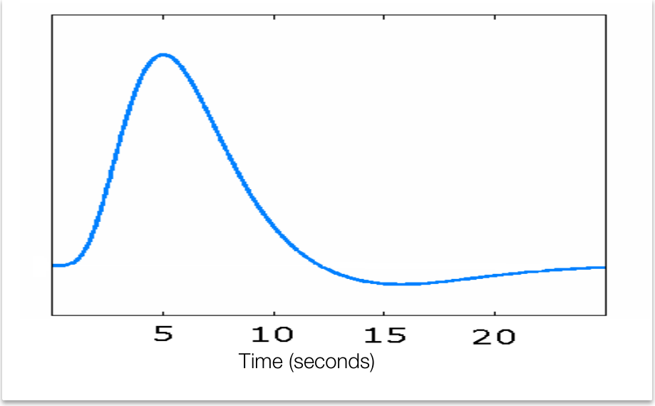
A canonical hemodynamic response function. A brief burst of neural activity at time zero produces a delayed BOLD response peaking around 5 seconds, followed by an undershoot below baseline before returning to equilibrium. (Figure 12.7 from the book. © the authors and MIT Press; reproduced with permission — not covered by this site’s CC-BY license.)
A widely used mathematical form for the canonical HRF is the difference of two gamma functions — one gamma creates the peak, and a second, later gamma subtracts to create the undershoot:
h(t) — HRF amplitude at time t · t — time since neural activity (s) · α₁, β₁ — shape and rate of the peak gamma · α₂, β₂ — shape and rate of the undershoot gamma · c — undershoot amplitude · Γ — gamma function
where is the hemodynamic response at time (seconds since neural activity), and are the shape and rate parameters of the gamma function that creates the peak, and the shape and rate of the later gamma that creates the undershoot, the relative amplitude of the undershoot, and the gamma function that normalizes each term.
Common parameter choices — the defaults in SPM — are , , , and , which place the peak near 5 seconds and the undershoot minimum near 15 seconds. Most studies assume this canonical shape holds for every voxel, task, and person — a simplification that buys tractable analysis. In reality the HRF varies across individuals; it becomes lower in amplitude and more protracted with age; and it is altered by caffeine, hypertension, diabetes, chronic alcohol use, and neurodegenerative disease — anything that affects the vasculature. It also varies across brain regions and task states, because different psychological events evoke neural responses with different durations and intensities: during memory encoding, for example, visual regions respond briefly while the hippocampus responds in a more sustained fashion. When the true response deviates from the assumed canonical form, the model is simply wrong for that voxel — a theme we revisit when we cover basis sets and flexible HRF models.
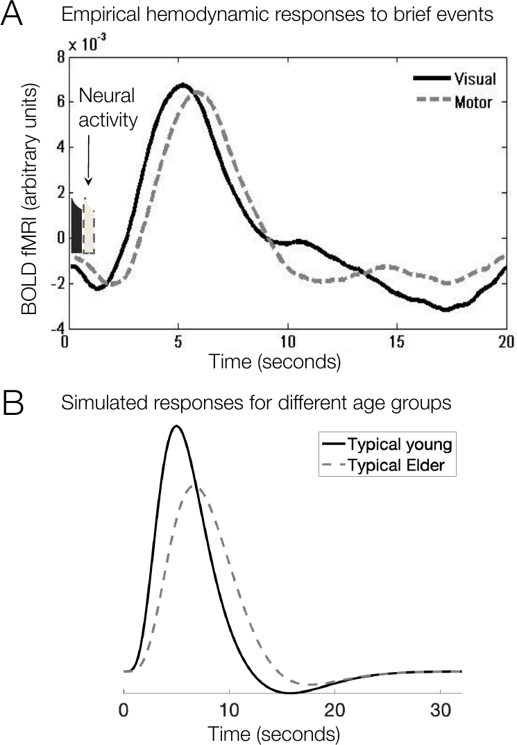
HRF shape is not fixed. Top: empirical HRFs to brief events, sampled every 100 ms, in visual and motor cortex — the initial dip, ~5 s peak, and undershoot are all visible, and the motor response lags the visual one. Bottom: simulated canonical (young) and elderly HRFs; with age the response becomes lower in amplitude and more protracted. (Figure 14.2 from the book. © the authors and MIT Press; reproduced with permission — not covered by this site’s CC-BY license.)
What, physiologically, drives the vasodilation? Both neurons and glia. Brain capillaries are lined by endothelial cells that form the blood–brain barrier, and astrocytes — glial cells with “end feet” that wrap those vessels — regulate their dilation and permeability. Vasodilation is triggered by multiple messengers: glutamate signaling (the brain’s dominant excitatory transmitter) induces release of vasodilatory nitric oxide and prostaglandins (PGE2), whereas GABA-ergic interneurons release vasoconstrictive neuropeptide Y and somatostatin. As rules of thumb, excitatory signaling tends to increase BOLD and inhibitory signaling can decrease it — but the rules are not absolute (optogenetically driving inhibitory interneurons can produce vasodilation and BOLD increases). Reassuringly, the bulk of evidence shows BOLD tracking local neural activity with impressive fidelity: BOLD responses follow local field potentials to within about 1 mm of peak electrical activity, correlate with markers of cellular activity and gamma-band synchrony, and closely mirror direct calcium imaging of neural activity in wide-field studies — including during spontaneous, resting-state fluctuations. BOLD decreases below baseline likewise often reflect genuine neural suppression in regions neighboring activated sites. One more wrinkle: diffuse neuromodulatory systems (dopaminergic VTA, noradrenergic locus coeruleus, cholinergic basal forebrain, serotonergic raphe) project broadly across the brain, and stimulating them — as opto- and chemo-fMRI studies do — can produce widespread BOLD changes. Widespread signal is therefore not automatically artifact, and local BOLD is not automatically local neuronal firing.
Finally, how do we relate BOLD to the mind? A powerful strategy is the dose–response relationship: BOLD in appropriate regions increases approximately linearly with stimulus intensity, cognitive demand, reaction time, subjective value, or pain — validating the signal against behavior much as pharmacology validates a drug against outcomes. But linearity has limits. Responses saturate: when stimuli of the same type repeat within a few seconds, later responses are reduced by refractory effects in both the neural and vascular response. Elevated baseline blood flow (from drugs, tonic states, or hypercapnia) can also blunt evoked responses. In practice, linearity is a good approximation for events spaced ~5 seconds or more apart and deteriorates below ~2 seconds — and, as you will see in the tutorial, unmodeled saturation doesn’t just add noise; it systematically biases amplitude estimates for closely spaced events. Because so many stable person-level factors (hematocrit, caffeine, vascular health, head motion) also shape BOLD amplitude, within-person brain–behavior relationships are generally far more robust than between-person correlations.
Hands-on tutorial
In this tutorial you will build the canonical HRF from gamma functions, use convolution to predict responses to brief events and sustained epochs, and then break the linear model on purpose — simulating vascular saturation to see how closely spaced stimuli under-add and bias GLM estimates.
Step 1 — Build a canonical HRF and convolve brief vs. sustained events. The double-gamma HRF is the impulse response of our assumed linear system; convolving it with a stimulus function predicts the BOLD response to any event sequence. Compare a 0.5-second event with a 20-second epoch.
% Requires CanlabCore + SPM12 on your MATLAB path
% Adapted from CANlab tutorials (github.com/canlab)
dt = 0.1;                                  % time resolution (s)
hrf = spm_hrf(dt); hrf = hrf ./ max(hrf);  % canonical double-gamma HRF
figure; plot((0:length(hrf)-1) * dt, hrf);
xlabel('Time (s)'); title('Canonical HRF');

% Brief event vs. sustained epoch, via onsets2fmridesign
TR = 1;                                    % repetition time / sampling interval (s)
len = 60;                                  % simulated run length (s)
ons = {};                                  % onsets: one cell per condition
ons{1} = [10 0.5];                         % onset 10 s, duration 0.5 s
ons{2} = [10 20];                          % onset 10 s, duration 20 s
X = onsets2fmridesign(ons, TR, len);       % convolves with canonical HRF

figure; plot(0:TR:len-1, X(:, 1:2), 'LineWidth', 2);
legend({'Brief event (0.5 s)' 'Epoch (20 s)'});
xlabel('Time (s)'); ylabel('Predicted BOLD');
import numpy as np, matplotlib.pyplot as plt
from scipy.stats import gamma
dt = 0.1 # time resolution (s)
t = np.arange(0, 32, dt) # HRF time grid: 0-32 s
hrf = gamma.pdf(t, 6) - gamma.pdf(t, 16) / 6 # canonical double-gamma HRF
hrf = hrf / hrf.max() # normalize: single-event peak = 1
frame = np.arange(0, 60, dt) # 60 s at 0.1 s resolution
brief = ((frame >= 10) & (frame < 10.5)).astype(float) # 0.5 s event
epoch = ((frame >= 10) & (frame < 30)).astype(float) # 20 s epoch
resp = lambda s: np.convolve(s, hrf)[:frame.size] * dt # LTI prediction
plt.plot(frame, resp(brief), label="Brief event (0.5 s)")
plt.plot(frame, resp(epoch), label="Epoch (20 s)")
plt.xlabel("Time (s)"); plt.ylabel("Predicted BOLD"); plt.legend()Example output:
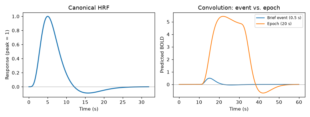
The canonical HRF (left) and the convolution predictions (right). The brief event produces a transient copy of the HRF; the 20 s epoch ramps up over ~10 s, plateaus while stimulation continues, then returns to baseline with an undershoot.
Step 2 — Nonlinear saturation for closely spaced events. Real BOLD responses under-add when events are packed together. We model this with a compressive “squashing” function applied to the linear prediction, and compare two events 1 second apart with the pure LTI prediction.
% Compressive saturation of the summed response
% (see also hrf_saturation.m and the 'nonlinsaturation' option
%  of onsets2fmridesign in CanlabCore)
cap = 2;                                   % ceiling, in single-event peak units
sat = @(x) cap .* tanh(x ./ cap);          % near-linear when small, squashed when large

ons2 = {}; ons2{1} = [20 21]';             % two events 1 s apart
X2 = onsets2fmridesign(ons2, TR, len);     % convolve with canonical HRF
x_lin = X2(:, 1);                          % linear (LTI) prediction

figure; plot(0:TR:len-1, x_lin, '--', 'LineWidth', 2); hold on;
plot(0:TR:len-1, sat(x_lin), 'LineWidth', 2);
legend({'Linear (LTI) prediction' 'With vascular saturation'});
xlabel('Time (s)'); ylabel('Response');
cap = 2.0 # ceiling, in single-event peak units
sat = lambda x: cap * np.tanh(x / cap) # near-linear when small, squashed when large
pair = np.zeros_like(frame) # two events 1 s apart
pair[(frame >= 20) & (frame < 20.5)] = 1
pair[(frame >= 21) & (frame < 21.5)] = 1
x_lin = resp(pair) / resp(brief).max() # linear prediction, single-event peak = 1
plt.plot(frame, x_lin, "--", label="Linear (LTI) prediction")
plt.plot(frame, sat(x_lin), label="With vascular saturation")
plt.xlabel("Time (s)"); plt.ylabel("Response"); plt.legend()Example output:
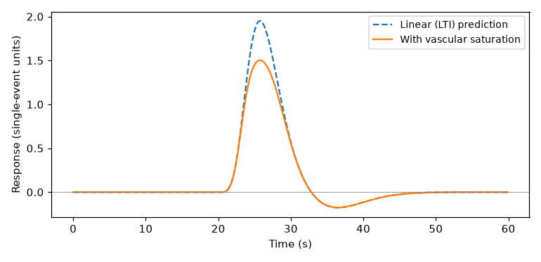
Two events 1 s apart: the linear model predicts a peak of ~1.95 single-event units, but with vascular saturation the response reaches only ~1.5 — the second event under-adds.
The saturated response falls short of the linear prediction exactly when predicted amplitude is high — that is, when events are dense. The full labs push this further: they map how the second event’s response shrinks as inter-stimulus interval drops from 12 s to 1 s, simulate a young vs. elderly HRF, and show that fitting a linear GLM to saturating data biases amplitude estimates downward for densely presented conditions relative to sparse ones — a design lesson as much as a physiology lesson.
Open the full Python lab notebook → or download the MATLAB live script, which mirrors it using CANlab tools.


Thought questions
You compare task activation between older adults with hypertension and healthy young controls, and find weaker BOLD responses in the patient group. Given that the HRF is shaped by both neural and vascular factors, what alternative explanations must you rule out before concluding the groups differ in neural processing — and what measurements or design choices (e.g., breath-hold calibration, within-person contrasts, flexible HRF models) could help disentangle them?
BOLD increases usually track excitatory activity, yet stimulating inhibitory interneurons can also produce vasodilation and BOLD increases, and “deactivations” can reflect true neural suppression. How should these facts change the language you use when interpreting a statistical map — and when is it defensible (or not) to call a negative BOLD response “inhibition”?
Opto- and chemo-fMRI show that stimulating neuromodulatory nuclei (VTA, locus coeruleus, basal forebrain) produces widespread, even near-global, BOLD changes. What does this imply for common preprocessing choices that remove global or widespread signals, and for interpreting distributed activation patterns in studies of arousal, attention, or drug effects?
Suppose your experiment compares a frequent “standard” stimulus with a rare “oddball,” so one condition’s events are far denser in time than the other’s. Using what you learned about refractory effects and vascular saturation, explain how a perfectly linear analysis could manufacture a spurious condition difference — and propose two remedies, one at the design stage and one at the modeling stage.
Within-person dose–response relationships between BOLD and behavior are typically much stronger than between-person correlations of the same variables. Drawing on the non-neural factors that vary across individuals, explain why — and what this implies for using fMRI as a biomarker of individual differences.
Quiz yourself
Q1. What property of hemoglobin makes BOLD imaging possible?
Answer: Oxygenated and deoxygenated hemoglobin differ magnetically: deoxyhemoglobin is paramagnetic, distorting the local field and shortening T2*, whereas oxygenated blood has a longer T2*. Changes in the relative concentration of the two therefore change T2*-weighted signal intensity, with no injected contrast agent needed.
Q2. What is neurovascular coupling?
Answer: The cascade linking neural activity to the vascular response: increased neural and glial signaling triggers oxygen extraction from hemoglobin and vasodilation, which increases local blood flow (and volume) in capillaries and arterioles. This coupling is what allows a hemodynamic signal to serve as a proxy for neural activity.
Q3. Describe the time course of the HRF following a brief burst of neural activity.
Answer: A small initial dip within about 0.5 s (rising deoxyhemoglobin lowers T2* signal), then a positive response beginning 1–2 s after onset and peaking 5–7 s after peak neural activity — roughly five times larger than the dip at 3 T — followed by a post-stimulus undershoot below baseline over the next ~10 s before returning to equilibrium.
Q4. What is a leading explanation for the post-stimulus undershoot?
Answer: Oxygen metabolism returns to baseline more slowly than blood flow and volume do, so after the flow response subsides, previously active tissue transiently contains a higher concentration of deoxyhemoglobin, pushing the signal below baseline. Buxton’s balloon model formalizes these flow–volume–metabolism dynamics.
Q5. Name the main cell types and chemical messengers that mediate vasodilation and vasoconstriction in neurovascular coupling.
Answer: Endothelial cells form the vessel walls (and blood–brain barrier); astrocyte end feet regulate them, alongside direct neuronal influences. Glutamatergic signaling drives release of vasodilators — nitric oxide and prostaglandins (PGE2) — while GABA-ergic interneurons release vasoconstrictors neuropeptide Y and somatostatin, with calcium signaling as a common pathway.
Q6. What evidence supports the claim that BOLD tracks local neural activity?
Answer: BOLD closely follows local field potentials (net synaptic activity), with increases within about 1 mm of peak electrical activity; it is associated with c-FOS expression and gamma-band synchrony; and it tracks direct calcium imaging of neural activity with high fidelity — including spontaneous resting-state fluctuations, where BOLD- and calcium-derived networks are remarkably similar.
Q7. Under what conditions does the linear (LTI) approximation for BOLD responses break down?
Answer: When events of the same type occur close together in time. Linearity holds reasonably well for events spaced roughly 5 s or more apart, but for spacings under about 2 s, refractory effects and saturation of the vascular response make responses to later stimuli substantially smaller than linear superposition predicts. Elevated baseline blood flow can also blunt evoked responses.
Q8. Why are within-person BOLD–behavior relationships generally more robust than between-person correlations?
Answer: Between-person comparisons are contaminated by stable non-neural differences — hematocrit, caffeine and other drug use, hypertension and vascular health, head motion — that alter BOLD amplitude independent of psychology. Within-person designs hold these factors largely constant, comparing conditions in the same brain and vasculature, which yields larger, more reliable effects.
 The book: Elements of Functional Magnetic Resonance Imaging — Wager & Lindquist, MIT Press