Fundamental MRI Physics
Run this code: ⚡ In-browser lab · Colab · MATLAB Online
Overview
MR scanners are remarkably versatile: the same machine can produce images of gross anatomy, white-matter pathways, blood flow, and moment-to-moment brain function. All of these rest on the same physical principles, and knowing a little of the physics goes a long way toward understanding what different image types actually measure. The story starts with the hydrogen nucleus — a single proton, chosen because of its favorable magnetic properties and its abundance in water, which makes up about 70% of the brain’s mass. Each proton behaves like a spinning charged sphere, generating a small magnetic moment along its axis; in MR physics these are called spins. A scanner never measures one spin — it measures the net magnetization of an enormous ensemble (roughly per gram of water), a vector with a longitudinal component parallel to the scanner’s main field and a transverse component perpendicular to it.
With no external field, the spins point in random directions and the net magnetization is zero. Inside the scanner’s field, a small majority align with , creating a net longitudinal magnetization, and each spin precesses about the field axis like a wobbling top. The precession rate, called the Larmor frequency, depends on the field strength and the type of nucleus — 127.74 MHz for hydrogen at 3T. It is also called the resonant frequency: spins absorb energy only when stimulated at precisely this frequency, and that resonance is the basis of all MR imaging. To measure the net magnetization, we must perturb the equilibrium and watch the system react. A radiofrequency (RF) pulse delivered at the Larmor frequency excites the spins: their phases become aligned with the pulse, which tips the net magnetization away from and establishes a transverse component rotating in the plane perpendicular to the field.
When the RF pulse ends, the system relaxes back to equilibrium along two separable dimensions, and the emitted energy induces the current in the head coil that constitutes the MR signal. Transverse relaxation is the loss of the transverse magnetization as spins dephase relative to one another, an exponential decay with time constant T2:
M_xy(t) — transverse magnetization remaining at time t · M₀ — equilibrium net magnetization · T₂ — transverse relaxation time constant (tissue-specific)
where is the transverse magnetization at time after the RF pulse ends, the equilibrium net magnetization, and the tissue-specific time constant of transverse decay.
Longitudinal relaxation is the recovery of magnetization along as spins re-align with the field, an exponential recovery with time constant T1:
M_z(t) — longitudinal magnetization recovered at time t · M₀ — equilibrium net magnetization · T₁ — longitudinal relaxation time constant (tissue-specific)
where is the longitudinal magnetization at time after excitation, the equilibrium net magnetization, and the tissue-specific time constant of longitudinal recovery.
Both constants have a “63% interpretation” that falls straight out of the math: at the longitudinal signal has recovered of its equilibrium value, and at the transverse signal has decayed to of its starting value. Crucially, T1 and T2 differ across tissue types — gray matter, white matter, and cerebrospinal fluid (CSF) each have characteristic values — and that difference is what makes anatomical contrast possible. A third constant, T2*, describes transverse decay that also includes dephasing from local field inhomogeneities. Deoxygenated hemoglobin is paramagnetic and distorts the local field, so T2* is sensitive to blood oxygenation and flow — the physical basis of functional imaging (Chapter 14).
Different image types are produced by pulse sequences — programmed patterns of RF excitation and readout — that emphasize different tissue properties. Two parameters do most of the work: TR (repetition time), how often we excite the spins, and TE (echo time), how long after excitation we collect data. A long TR with a short TE makes the signal proportional simply to the number of protons, yielding a proton-density image. An intermediate TR with a short TE yields a T1-weighted image, in which white matter is brightest, gray matter intermediate, and CSF dark. A long TR with an intermediate TE yields a T2-weighted image, in which CSF is brightest — and in which pathology such as demyelination, inflammation, and tumors appears bright, which is why T2-weighted scans are a clinical workhorse. T2*-weighted images use similar timing to T2-weighted ones but differ in how the gradients are used, and their sensitivity to deoxyhemoglobin makes them the basis for fMRI.
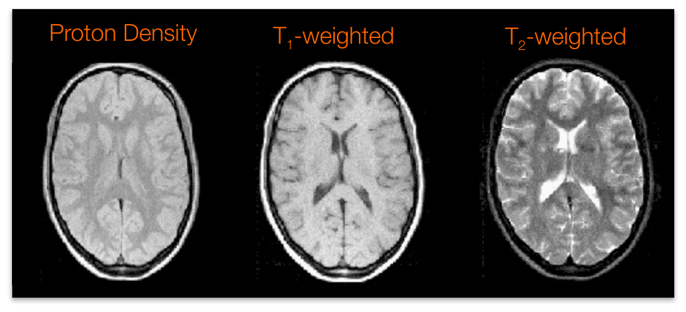
The same brain, three contrasts. Proton density (left) reflects water content and shows relatively uniform brain tissue. In the T1-weighted image (middle), white matter is bright and CSF-filled ventricles are dark. In the T2-weighted image (right), the pattern reverses: CSF is bright and white matter is dark. (From the book’s companion slides for Chapter 13. © the authors and MIT Press; reproduced with permission — not covered by this site’s CC-BY license.)
Turning excited spins into a picture is the problem of image formation. Most MRIs are acquired as a stack of 2D slices (sequentially or interleaved), and exciting a slice tells us only its total magnetization. To recover each voxel’s contribution, three gradient coils impose controlled linear variations on the magnetic field: one gradient selects the slice, and the other two perform frequency and phase encoding. Each measurement then corresponds to the Fourier transform of the slice’s signal at one spatial frequency — one coordinate in k-space. Standard sequences such as echo-planar imaging (EPI) sample k-space line by line; once enough of k-space is covered, an inverse fast Fourier transform reconstructs the image. Because the Fourier transform is reversible, image space and k-space are two complete representations of the same data. Each k-space point encodes a 2D sinusoid spread across the entire image: its distance from the k-space center sets the sinusoid’s spatial frequency (center = coarse, smooth structure; periphery = fine detail and edges), and its polar angle sets the orientation. The raw k-space data are complex-valued; reconstruction yields magnitude and phase images, and nearly all fMRI analyses use only the magnitude.
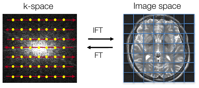
k-space and image space are linked by the Fourier transform (FT) and its inverse (IFT). The scanner measures spatial frequencies — typically one line of k-space at a time (arrows) — and the inverse transform reconstructs the voxel-by-voxel image. (From the book’s companion slides for Chapter 13. © the authors and MIT Press; reproduced with permission — not covered by this site’s CC-BY license.)
Finally, measuring brain function means acquiring T2*-weighted volumes repeatedly — one every TR, traditionally about 2 s (with modern multiband/simultaneous multi-slice sequences pushing much faster) — while the participant performs a task or rests. Structural (T1- or T2-weighted) scans give exquisite anatomical detail but are a single snapshot in time; functional (T2*-weighted) scans trade spatial detail for a time series, letting us test how the signal changes with experimental conditions. That link between T2* changes and neuronal activity is the subject of the next chapter.
Hands-on tutorial
The physics above reduces to a handful of equations you can explore directly. In this tutorial you will plot T1 recovery and T2 decay for different tissues, and then take an image apart in k-space. The full labs also build a digital head phantom and use the MR signal equation to generate PD-, T1-, and T2-weighted images from the same “brain”:
S — measured signal · ρ — proton density (number of contributing hydrogen nuclei) · TR — repetition time · TE — echo time · T₁, T₂ — tissue relaxation time constants
where is the measured signal from a tissue, its proton density (the number of contributing hydrogen nuclei), the repetition time, the echo time, and , its relaxation time constants.
Step 1 — Plot T1 recovery curves for gray matter, white matter, and CSF. Each tissue recovers at its own rate; at , each curve crosses 63% of full recovery.
% Adapted from CANlab tutorials (canlab.github.io, Lab 1: T1 decay)
t = 1:4000;                                   % time after excitation (ms)
t1relax = @(t, T1) 1 - exp(-t ./ T1);         % T1 recovery function

figure; hold on;
plot(t, t1relax(t, 1000), 'LineWidth', 3);    % gray matter, T1 = 1000 ms
plot(t, t1relax(t, 600),  'LineWidth', 3);    % white matter, T1 = 600 ms
plot(t, t1relax(t, 3000), 'LineWidth', 3);    % CSF,          T1 = 3000 ms
plot([0 4000], [1 - 1/exp(1), 1 - 1/exp(1)], 'k--');  % 63% recovery line
xlabel('Time (ms)'); ylabel('M_z / M_0');
title('T1 (longitudinal) relaxation');
legend({'Gray', 'White', 'CSF', '63%'}, 'Location', 'southeast');
import numpy as np
import matplotlib.pyplot as plt
t = np.arange(0, 4000) # time after excitation (ms)
t1relax = lambda t, T1: 1 - np.exp(-t / T1) # T1 recovery function
fig, ax = plt.subplots(figsize=(6, 4)) # figure size in inches
for T1, name in [(1000, "Gray"), (600, "White"), (3000, "CSF")]: # T1 per tissue (ms)
ax.plot(t, t1relax(t, T1), lw=3, label=f"{name} (T1={T1} ms)")
ax.axhline(1 - 1 / np.e, color="k", ls="--", label="63% recovery")
ax.set(xlabel="Time (ms)", ylabel="$M_z / M_0$",
title="T1 (longitudinal) relaxation")
ax.legend(loc="lower right")Example output:
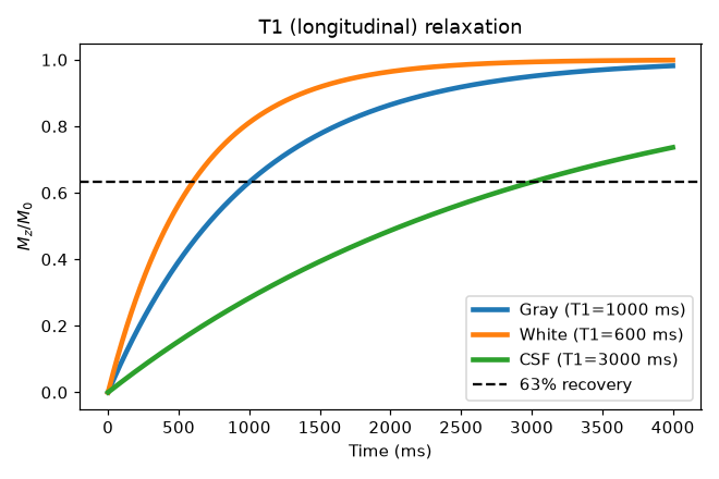
Output of Step 1: each tissue’s longitudinal magnetization recovers exponentially and crosses the dashed 63% line at its own — white matter first (600 ms), then gray matter (1000 ms), then CSF (3000 ms).
At any single readout time, the three tissues sit at different heights on their curves — that vertical separation is the T1 contrast, and TR controls where on the curves you sample. (T2 decay works the same way, with and TE.)
Step 2 — Take an image into k-space, and knock out the center or the edges. The 2D FFT converts an image to k-space and back. Keeping only the center keeps the smooth, low-frequency structure; keeping only the edges keeps fine detail.
% Simple head phantom: gray shell, white interior, CSF ventricles
n = 128;                                      % image matrix size (n-by-n voxels)
[x, y] = meshgrid(linspace(-1, 1, n));        % voxel coordinate grids on [-1, 1]
img = zeros(n);
img((x/0.72).^2 + (y/0.92).^2 < 1) = 0.30;    % gray-matter shell
img((x/0.52).^2 + (y/0.72).^2 < 1) = 0.35;    % white-matter interior
img(((x+0.13)/0.09).^2 + ((y+0.05)/0.33).^2 < 1) = 0.15;  % ventricles
img(((x-0.13)/0.09).^2 + ((y+0.05)/0.33).^2 < 1) = 0.15;

F = fftshift(fft2(img));                      % image -> k-space
[kx, ky] = meshgrid((1:n) - n/2 - 1);         % k-space coordinate grids
center = sqrt(kx.^2 + ky.^2) < 10;            % keep radius < 10 (of 64): low spatial frequencies

subplot(1, 4, 1); imagesc(img); axis image off; title('Image');
subplot(1, 4, 2); imagesc(log(1 + abs(F))); axis image off; title('k-space');
subplot(1, 4, 3); imagesc(abs(ifft2(ifftshift(F .* center))));
axis image off; title('Center only');
subplot(1, 4, 4); imagesc(abs(ifft2(ifftshift(F .* ~center))));
axis image off; title('Edges only');
colormap gray;
# Simple head phantom: gray shell, white interior, CSF ventricles
n = 128 # image matrix size (n x n voxels)
y, x = np.mgrid[-1:1:n*1j, -1:1:n*1j] # voxel coordinate grids on [-1, 1]
img = np.zeros((n, n))
img[(x/0.72)**2 + (y/0.92)**2 < 1] = 0.30 # gray-matter shell
img[(x/0.52)**2 + (y/0.72)**2 < 1] = 0.35 # white-matter interior
img[((x+0.13)/0.09)**2 + ((y+0.05)/0.33)**2 < 1] = 0.15 # ventricles
img[((x-0.13)/0.09)**2 + ((y+0.05)/0.33)**2 < 1] = 0.15
F = np.fft.fftshift(np.fft.fft2(img)) # image -> k-space
ky, kx = np.mgrid[-n//2:n//2, -n//2:n//2] # k-space coordinate grids
center = np.sqrt(kx**2 + ky**2) < 10 # keep radius < 10 (of 64): low spatial frequencies
fig, axes = plt.subplots(1, 4, figsize=(12, 3.2)) # 4 panels side by side
panels = [(img, "Image"), (np.log1p(np.abs(F)), "k-space"),
(np.abs(np.fft.ifft2(np.fft.ifftshift(F * center))), "Center only"),
(np.abs(np.fft.ifft2(np.fft.ifftshift(F * ~center))), "Edges only")]
for ax, (im, name) in zip(axes, panels):
ax.imshow(im, cmap="gray"); ax.set_title(name); ax.axis("off")Example output:
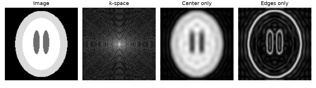
Output of Step 2: the phantom (left), its log-magnitude k-space (bright at the center), the smooth low-frequency reconstruction from the center of k-space, and the edge-only reconstruction from the periphery.
Notice the bright blob at the middle of k-space: most of the image’s energy lives in a few low spatial frequencies. The “center only” reconstruction is a blurry but recognizable brain, while the “edges only” reconstruction contains just outlines — exactly the division of labor described in the overview. The full labs go on to build T1- and T2-weighted versions of this phantom from the signal equation and to show how a single k-space point maps to stripes across the whole image.
Open the full Python lab notebook → or download the MATLAB live script, which mirrors it and extends the CANlab “T1 decay” tutorial.


Thought questions
Hydrogen is imaged because it is magnetically favorable and abundant. Suppose you wanted to image a different nucleus (e.g., P or Na) present at far lower concentrations. Reasoning from net magnetization and signal-to-noise, what would you expect to happen to achievable spatial resolution and scan time, and why?
Using the signal equation , explain why a long TR combined with a short TE removes both T1 and T2 influences, leaving a proton-density image. Then explain what would happen to tissue contrast if you chose a very long TE together with a very short TR — why is that combination never used?
fMRI relies on T2*, not T2. What extra physical process does T2* capture, and how does that same process explain both the usefulness of T2*-weighted images for measuring brain function and their vulnerability to signal dropout near air-filled sinuses?
A participant moves their head briefly during a structural scan. Predict how the artifact would differ depending on whether the motion occurred while the scanner was sampling the center of k-space versus its outer edges, and justify your prediction from the information content of each region.
Accelerated acquisitions (partial k-space, parallel imaging, multiband) all involve measuring fewer k-space samples per unit time. What is fundamentally being traded away, and why can clever reconstruction recover much — but never all — of it?
Quiz yourself
Q1. Why are hydrogen nuclei the standard target for MRI?
Answer: Hydrogen (H, a single proton) has favorable magnetic properties and is extremely abundant in the body, because water — about 70% of the brain’s mass — contains hydrogen. This abundance yields a large net magnetization and hence a measurable signal.
Q2. What happens to nuclear spins when a person is placed inside the scanner’s field, before any RF pulse is applied?
Answer: A small majority of spins align with the field (low-energy state) rather than against it, creating a net longitudinal magnetization along . The spins precess about the field axis at the Larmor frequency, but with random phases, so there is no net transverse magnetization.
Q3. What is the Larmor frequency, and what two factors determine it?
Answer: It is the frequency at which spins precess about the main magnetic field — and the resonant frequency at which they absorb RF energy and become excited. It depends on the strength of the magnetic field () and the type of nucleus; for hydrogen at 3T it is 127.74 MHz.
Q4. Define T1 and T2 relaxation, including the “63%” interpretation of each constant.
Answer: T1 (longitudinal) relaxation is the exponential recovery of magnetization along as spins re-align with the field; T1 is the time to recover 63% () of the equilibrium value. T2 (transverse) relaxation is the exponential loss of transverse magnetization as spins lose phase coherence; T2 is the time for the signal to fall by 63%, i.e., to of its initial value.
Q5. How do T2 and T2* differ, and why does the difference matter for fMRI?
Answer: T2* includes everything in T2 plus additional dephasing caused by local magnetic field inhomogeneities. Deoxygenated hemoglobin is paramagnetic and distorts the local field, so T2* is sensitive to blood oxygenation and flow — which is what makes T2*-weighted imaging the basis of functional MRI.
Q6. Match the TR/TE combinations to the image types: (a) long TR + short TE, (b) intermediate TR + short TE, (c) long TR + intermediate TE.
Answer: (a) Proton-density image — signal proportional to the number of protons. (b) T1-weighted image — contrast dominated by differences in T1 recovery. (c) T2-weighted image — contrast dominated by differences in T2 decay (T2*-weighted functional images use similar timing but different gradient usage).
Q7. On a T1-weighted image, rank gray matter, white matter, and CSF from brightest to darkest. How does the ranking change on a T2-weighted image, and why are T2-weighted scans popular clinically?
Answer: T1-weighted: white matter brightest, then gray matter, with CSF darkest. T2-weighted: CSF brightest, with gray and white matter darker (white matter darkest). Pathology such as demyelination, inflammation, and tumors appears bright on T2-weighted images, making them especially useful in clinical settings.
Q8. What information do the center and the periphery of k-space carry, and what operation converts fully sampled k-space into an image?
Answer: Each k-space point encodes a 2D sinusoid across the whole image; points near the center encode low spatial frequencies (coarse structure and most of the image’s energy), while points far from the center encode high spatial frequencies (fine detail and edges), with orientation given by the polar angle. An inverse Fourier transform (in practice the inverse FFT) reconstructs the image.
 The book: Elements of Functional Magnetic Resonance Imaging — Wager & Lindquist, MIT Press