Spatial and Temporal Resolution
Run this code: ⚡ In-browser lab · Colab · MATLAB Online
Overview
Much of what can — and cannot — be inferred from an fMRI study traces back to its spatial and temporal resolution. Spatial resolution refers to the size of the voxels used to construct an image, and describes the ability to distinguish signal changes across anatomical locations. Temporal resolution describes the ability to distinguish signal changes across time points. Because data collection speed is limited, the two trade off against each other, and both are further constrained by the biophysics of the BOLD response itself.
Spatial resolution matters because neurons with similar functional properties tend to cluster anatomically, at scales ranging from whole-brain networks (centimeters) down to cortical columns (0.1–2 mm) and single cells (5–100 μm). Modern 3T studies typically acquire ~3 mm voxels, and high-field (7T) imaging can go below 1 mm — enough to reach a great deal of functionally meaningful structure. The thalamus, for example, contains over 30 nuclei per hemisphere averaging about 6.5 mm in diameter, comfortably within reach of standard fMRI. The finer the scale of interest, the more the analysis strategy matters: group analyses are sensitive to regions and networks, individual-subject analyses can localize signal down to 1–2 mm, and multivariate pattern analysis (MVPA) within individuals may pick up information encoded at even finer scales.
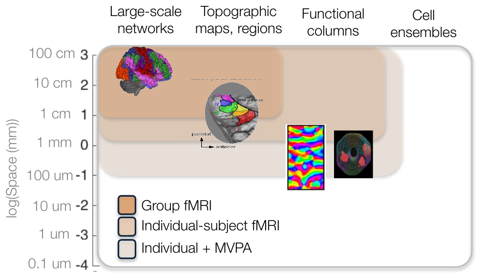
The brain encodes psychological and behavioral information at multiple spatial scales, from large-scale networks (2–100 cm) through topographic maps and regions (1 mm–2 cm) and functional columns (100 μm–2 mm) down to cell ensembles and single neurons. Group fMRI is sensitive to the coarser scales; individual-subject analyses and MVPA extend sensitivity toward finer ones. (Figure 15.1 from the book. © the authors and MIT Press; reproduced with permission — not covered by this site’s CC-BY license.)
Given all that structure, why not simply acquire the smallest voxels the scanner allows? Three costs push back. First, the signal-to-noise ratio (SNR) of a voxel is proportional to its volume — halving each side of a 3 mm voxel cuts its volume, and thus its intrinsic SNR, by a factor of eight. Second, higher-resolution images take longer to acquire, degrading temporal resolution and increasing motion-related artifacts. Third, at the other extreme, voxels that are too large average over many neural populations and tissue types, diluting the signal from any one of them — the partial volume effect — and are more prone to susceptibility artifacts where they span tissue boundaries. The optimal voxel size balances these costs.
Even a perfectly chosen voxel size overstates what a study can resolve. The effective resolution is limited by the physiology of the BOLD response, which arises in arterioles and capillary beds and spreads into draining veins beyond the site of neural activity. This blurring is summarized by the BOLD point-spread function: roughly 3.5 mm at 3T and as low as ~1.5 mm at 7T, so there may be limited benefit in acquiring voxels much smaller than these values. Analysis choices erode resolution further, especially for group studies. Warping individual brains to a common template (e.g., MNI space) leaves substantial residual misalignment — functional areas like MT or the fusiform face area can vary in location by 2 cm or more across people — and spatial smoothing, applied partly to compensate, blurs the maps again. Reporting peak coordinates costs still more: across comparable group studies, peak locations for the same effect vary by roughly 2–3 cm. Approaches that localize regions or patterns of interest within individual participants, and functional alignment methods such as hyperalignment, preserve much more of the acquired resolution — including “hyperacuity” effects in which multivariate patterns capture information (e.g., ocular dominance) encoded at scales finer than the voxels themselves.
On the temporal side, fMRI is coarse compared with EEG or MEG. The sampling rate is set by the TR (typically 0.5–3 s), but the deeper limit is the hemodynamic response itself, which begins ~2 s after a brief event and peaks at 5–6 s. A TR of 2 s has therefore long been considered “adequate” — yet slow sampling carries real costs. The Nyquist theorem states that a periodic signal can only be resolved if it is sampled at more than twice its frequency; with sampling frequency , the highest resolvable frequency is
f_Nyquist — highest resolvable frequency (Hz) · F_s — sampling frequency (Hz, volumes per second) · TR — repetition time (s, time between volumes)
where is the highest frequency that can be resolved, the sampling frequency (volumes per second), and the repetition time in seconds.
Any signal above this limit does not disappear — it is reflected (folded) back around the Nyquist frequency and masquerades as a lower-frequency signal, a phenomenon called aliasing. A 1 Hz heartbeat sampled at TR = 0.5 s ( Hz) stays at its own frequency, well above the slow task-related band, where it can be filtered out. The same heartbeat sampled at TR = 2 s ( Hz) is aliased into the low frequencies where task effects live, becoming inseparable from activation. Physiological noise is the largest noise source in fMRI and a major source of temporal autocorrelation, so aliased cardiac and respiratory signals are particularly damaging — for task analyses and even more so for functional connectivity. Slow sampling has a second cost: if event onsets are locked to the TR, the response peak can fall between samples. Presenting events at variable times relative to the TR oversamples the hemodynamic response and avoids this bias.
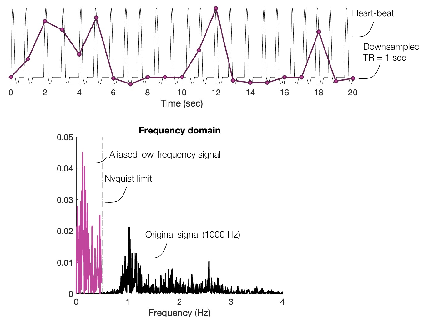
Aliasing of physiological noise. Top: a simulated heartbeat at 60 beats per minute (black) sampled at TR = 1 s (purple). Bottom: in the frequency domain, cardiac power above the Nyquist limit (dashed line at Hz) is folded back into the low temporal frequencies where task-related signal resides. (Figure 16.6 from the book. © the authors and MIT Press; reproduced with permission — not covered by this site’s CC-BY license.)
Designing an acquisition protocol means balancing four desirable properties — brain coverage, spatial resolution, temporal resolution, and freedom from artifacts — where improving one generally costs another. Whole-brain coverage at ~4 mm slice thickness takes about 2 s with standard protocols; better spatial or temporal resolution can be bought by reducing coverage, or by accelerated imaging: in-plane acceleration (skipping lines of k-space, with multi-coil reconstruction correcting the resulting aliasing artifacts) and multiband / simultaneous multi-slice (SMS) imaging, which excites and reads multiple slices at once. Multiband can reduce whole-brain TRs from ~2 s to a few hundred milliseconds — a current recommended standard is ~3 mm isotropic voxels, whole-brain, at TR < 1 s (e.g., multiband factor 6) — though each image is noisier, and aggressive acceleration can reduce contrast-to-noise and BOLD sensitivity. Many groups now push TR below 500 ms specifically to keep physiological signals below the Nyquist limit. Adopting a well-piloted standard protocol (e.g., harmonized with the Human Connectome Project or ABCD studies) reduces guesswork and aids comparability across studies.
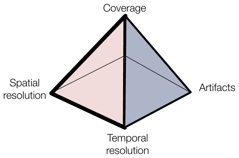
fMRI acquisition involves tradeoffs among brain coverage, spatial resolution, temporal resolution, and absence of artifacts: parameter choices that improve one generally cost another. (Figure 15.2A from the book. © the authors and MIT Press; reproduced with permission — not covered by this site’s CC-BY license.)
Hands-on tutorial
The labs make these tradeoffs concrete with simulations. Here are two key steps: aliasing a “heartbeat” by sampling it at a typical TR, and smoothing small versus large activations.
Step 1 — Alias a heartbeat by sampling at the TR. We simulate a cardiac signal at 66 beats per minute (1.1 Hz) and sample it once per TR. At TR = 0.4 s the Nyquist limit ( Hz) is above the cardiac frequency and the peak stays at 1.1 Hz; at TR = 2 s ( Hz) it is aliased to 0.1 Hz — right into the task band.
% Adapted from CANlab tutorials (canlab.github.io) and
% github.com/canlab/FMRI_simulations
fs = 1000;                           % fs = simulation sampling rate (Hz) for "ground truth"
t = 0:1/fs:60-1/fs;                  % t = time vector, 60 s long
heart = sin(2*pi*1.1*t);             % simulated heartbeat: 66 bpm = 1.1 Hz

for TR = [0.4 2.0]                   % TR = time between volumes (s): fast vs. typical
    samp = heart(1:round(TR*fs):end);    % sample once per TR, like the scanner
    n = numel(samp);                     % n = number of samples (volumes)
    f = (0:floor(n/2)) ./ (n*TR);        % frequencies up to Nyquist
    p = abs(fft(samp)) / n;  p = p(1:floor(n/2)+1);
    [~, imax] = max(p);
    fprintf('TR = %.1f s: Nyquist = %.2f Hz, spectral peak at %.2f Hz\n', ...
        TR, 1/(2*TR), f(imax));
end
import numpy as np
fs = 1000 # fs = simulation sampling rate (Hz) for "ground truth"
t = np.arange(0, 60, 1 / fs) # t = time vector, 60 s long
heart = np.sin(2 * np.pi * 1.1 * t) # simulated heartbeat: 66 bpm = 1.1 Hz
for TR in (0.4, 2.0): # TR = time between volumes (s): fast vs. typical
samp = heart[::round(TR * fs)] # sample once per TR, like the scanner
freqs = np.fft.rfftfreq(len(samp), d=TR) # frequencies up to Nyquist
power = np.abs(np.fft.rfft(samp)) / len(samp)
print(f"TR = {TR} s: Nyquist = {1/(2*TR):.2f} Hz, "
f"spectral peak at {freqs[np.argmax(power)]:.2f} Hz")Example output:
TR = 0.4 s: Nyquist = 1.25 Hz, spectral peak at 1.10 Hz
TR = 2.0 s: Nyquist = 0.25 Hz, spectral peak at 0.10 Hz
Step 2 — Smooth small vs. large activations. A 1-D “cortical strip” (1 voxel = 1 mm) contains two activations of equal amplitude: one narrow (~3.5 mm FWHM, the scale of a small nucleus or column cluster) and one broad (~19 mm). Smoothing with a typical 8 mm FWHM Gaussian kernel suppresses noise and preserves the broad activation, but flattens the narrow one — smoothing is a matched filter that favors signals at its own scale.
rng(1);                                    % seed for reproducible noise
x = (1:200)';                              % position along the strip: 1 voxel = 1 mm
small = 2*exp(-(x - 60).^2 / (2*1.5^2));   % narrow activation: ~3.5 mm FWHM, amplitude 2
large = 2*exp(-(x - 140).^2 / (2*8^2));    % broad activation: ~19 mm FWHM, amplitude 2
y = small + large + randn(200, 1);         % add Gaussian noise, sd = 1

fwhm = 8;                                  % fwhm = smoothing kernel FWHM (mm), a typical choice
sig = fwhm / (2*sqrt(2*log(2)));           % convert FWHM -> Gaussian sigma
kern = exp(-(-20:20).^2 / (2*sig^2))';  kern = kern / sum(kern);
ysmooth = conv(y, kern, 'same');

figure; plot(x, y, 'Color', [.7 .7 .7]); hold on
plot(x, ysmooth, 'k', 'LineWidth', 2)
plot(x, small + large, 'r--')
legend({'Noisy data' 'Smoothed (8 mm FWHM)' 'True signal'})
xlabel('Position (mm)')
from scipy.ndimage import gaussian_filter1d
import matplotlib.pyplot as plt
rng = np.random.default_rng(1) # seed for reproducible noise
x = np.arange(200) # position along the strip: 1 voxel = 1 mm
small = 2 * np.exp(-(x - 60)**2 / (2 * 1.5**2)) # narrow activation: ~3.5 mm FWHM, amplitude 2
large = 2 * np.exp(-(x - 140)**2 / (2 * 8**2)) # broad activation: ~19 mm FWHM, amplitude 2
y = small + large + rng.standard_normal(200) # add Gaussian noise, sd = 1
fwhm = 8 # fwhm = smoothing kernel FWHM (mm), a typical choice
sigma = fwhm / (2 * np.sqrt(2 * np.log(2))) # convert FWHM -> Gaussian sigma
y_smooth = gaussian_filter1d(y, sigma)
plt.plot(x, y, color=".7", label="Noisy data")
plt.plot(x, y_smooth, "k", lw=2, label="Smoothed (8 mm FWHM)")
plt.plot(x, small + large, "r--", label="True signal")
plt.xlabel("Position (mm)"); plt.legend()Example output:
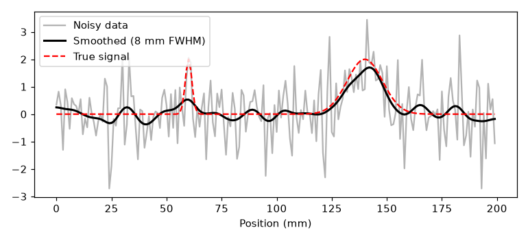
The 8 mm kernel preserves the broad (~19 mm) activation almost intact but flattens the narrow (~3.5 mm) one to a fraction of its true amplitude.
The full labs go further: building intuitions for sine waves and the FFT, aliasing a realistic spiky heartbeat with beat-to-beat variability, mapping which TRs keep cardiac signal separable from task frequencies, and quantifying how smoothing changes peak amplitude and SNR as a function of activation size.
Open the full Python lab notebook → or download the MATLAB live script, which mirrors it using CANlab-style idioms.


Thought questions
You are planning two studies: one mapping responses across the ~30 nuclei of the thalamus (average diameter ~6.5 mm), the other decoding line orientation from columns in V1 (~1 mm scale). For each, choose a voxel size, field strength, coverage, and analysis strategy (group mapping, individual ROI localization, or MVPA), and justify each choice using SNR-per-voxel, partial volume effects, and the BOLD point-spread function.
A colleague argues: “The hemodynamic response peaks at 5–6 seconds, so there is no point sampling faster than TR = 2 s.” Drawing on aliasing, motion within volumes, HRF estimation, and per-image SNR, make the strongest case for and against a TR under 500 ms.
Effective resolution is set by the weakest link in a chain running from physiology (point-spread) through acquisition (voxel size) to analysis (normalization, smoothing, peak reporting, ROI averaging). For a standard group study — 3 mm voxels, MNI normalization, 8 mm smoothing, peak-coordinate tables — identify the weakest link, and describe which links you would change first to improve it, at what cost.
Smoothing acts as a matched filter: it boosts sensitivity to signals at its own spatial scale while attenuating finer ones. Given that the extent of true activations is usually unknown and varies across regions, how should a researcher choose a smoothing kernel — or should they smooth at all? Consider group alignment, partial volume effects, and the alternative of multivariate analyses on unsmoothed data.
MVPA can detect ocular dominance information using 2–3 mm voxels, even though the columns themselves are ~1 mm wide (“fMRI hyperacuity”). Explain how information at a scale finer than the voxel grid can survive sampling, and why group-average univariate maps of the same data would miss it.
Quiz yourself
Q1. What do spatial resolution and temporal resolution refer to in fMRI?
Answer: Spatial resolution is the size of the voxels used to construct the image — the ability to distinguish signal changes across anatomical locations. Temporal resolution is the ability to distinguish signal changes across time points, set primarily by the TR.
Q2. Give two reasons not to simply acquire the smallest voxels the scanner allows.
Answer: SNR is proportional to voxel volume, so very small voxels have low intrinsic SNR; and higher-resolution images take longer to acquire, hurting temporal resolution and increasing motion-related artifacts.
Q3. What are partial volume effects?
Answer: When a voxel is large enough to span multiple neural populations or tissue types, the signal from any one population is diluted by averaging with the others. Large voxels crossing tissue boundaries also increase susceptibility artifacts.
Q4. What is the BOLD point-spread function, and roughly how large is it at 3T and at 7T?
Answer: It characterizes how much a point of neural activity is blurred in the BOLD image, because the hemodynamic response extends into adjacent vessels and draining veins. It is roughly 3.5 mm at 3T and as low as ~1.5 mm at 7T — so voxels much smaller than these values yield limited additional benefit.
Q5. State the Nyquist theorem and compute the Nyquist limit for TR = 2 s. What happens to a 1 Hz heartbeat signal at this TR?
Answer: A periodic signal can be resolved only if sampled at more than twice its frequency; the Nyquist limit is . For TR = 2 s the limit is 0.25 Hz, so a 1 Hz cardiac signal is aliased — folded back below the Nyquist limit into the low frequencies occupied by task-related signal, where it cannot be separated from activation.
Q6. Why is aliased physiological noise especially harmful for fMRI analyses?
Answer: Physiological noise is the largest source of noise in fMRI and contributes to temporal autocorrelation. Once aliased into task frequencies it cannot be filtered out without also removing task signal, and it can badly contaminate functional connectivity analyses, which are very sensitive to shared physiological fluctuations.
Q7. Why should event onsets not be locked to the TR, and what is the recommended alternative?
Answer: If events always start at the same point in the acquisition cycle, the HRF is sampled at the same phases each trial, and the response peak can fall between samples, underestimating amplitude. Presenting events at variable times relative to the TR oversamples the HRF (e.g., effective resolution TR/2 with two offsets), and regression is then used to estimate the response.
Q8. What is multiband (simultaneous multi-slice) imaging, and what tradeoff does it involve?
Answer: Multiband/SMS excites and acquires several slices at once, using many receive coils and special encoding to unmix them. It can cut whole-brain TR from ~2 s to a few hundred milliseconds, reducing aliased physiological noise — but each image is of lower quality, with potential costs in CNR and BOLD sensitivity, and combining SMS with in-plane acceleration can compound sensitivity to head motion.
 The book: Elements of Functional Magnetic Resonance Imaging — Wager & Lindquist, MIT Press