This lab builds hands-on intuition for the temporal and spatial resolution limits discussed in Chapter 15. You will construct sine waves and examine them with the fast Fourier transform (FFT), watch a fast signal get aliased to a slow one when sampled below the Nyquist limit, alias a simulated heartbeat by sampling it at typical fMRI TRs, and measure what spatial smoothing does to small versus large activations.
How to run this notebook. It runs anywhere with a standard scientific Python stack: directly
in the browser on the tutorial site, in Google Colab (badge on the chapter page), or locally
(numpy, scipy, and matplotlib are the only requirements). All data are simulated. Run the
cells top to bottom.
▶ This notebook is interactive. Click the ⏻ power icon at the top right of this page to run it in your browser — no installation needed (the kernel takes ~30–60 s to start the first time). Then run cells top to bottom, starting with the first code cell below: later cells depend on the imports and variables defined earlier, and will error if you skip ahead.
import numpy as np
import matplotlib.pyplot as plt
from scipy.ndimage import gaussian_filter1d

rng = np.random.default_rng(2026)   # seed for reproducible simulations
plt.rcParams.update({"figure.figsize": (9, 4), "axes.spines.top": False,
                     "axes.spines.right": False})
1. Sine waves and the FFT
A sine wave is defined by its frequency (cycles per second, Hz), amplitude, and phase
: . We simulate one at a high sampling frequency
Fs — think of this as the “ground truth” signal before the scanner samples it.
The FFT re-expresses a time-domain signal as a sum of sine waves of different frequencies. The magnitude of the (complex) Fourier coefficients tells us how much power the signal has at each frequency. The highest frequency that can be represented is the Nyquist limit, .
Adapted from the CANlab “Signal basics, fft, and aliasing” tutorial (canlab.github.io).
Fs = 1000                 # sampling frequency (samples/sec)
L = 1000                  # length of signal (samples) -> 1 second
t = np.arange(L) / Fs     # time vector (sec)

F = 10                    # frequency of the sine wave (Hz)
theta = 0                 # phase (radians)
y = np.sin(2 * np.pi * F * t + theta)

freqs = np.fft.rfftfreq(L, d=1 / Fs)   # frequencies for each FFT coefficient
mag = np.abs(np.fft.rfft(y)) / L       # magnitude spectrum

fig, axes = plt.subplots(1, 2, figsize=(10, 3.5))
axes[0].plot(t, y)
axes[0].set(xlabel="Time (sec)", ylabel="Signal", title=f"{F} Hz sine wave (time domain)")
axes[1].plot(freqs, mag)
axes[1].set(xlabel="Frequency (Hz)", ylabel="Magnitude", xlim=(0, 50),
            title="Magnitude spectrum (frequency domain)")
axes[1].axvline(F, color="r", ls=":", alpha=0.5)
plt.tight_layout()

print(f"Nyquist limit = Fs/2 = {Fs / 2:.0f} Hz")
Nyquist limit = Fs/2 = 500 Hz
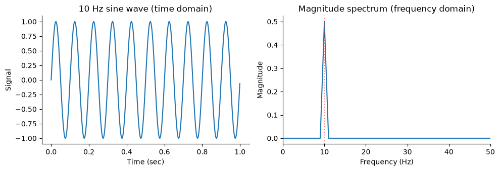
The spectrum shows a single sharp peak at 10 Hz — all of this signal’s power lives at one
frequency. Try it: change F to 20, or set theta = np.pi / 2 (which turns the sine into a
cosine). The peak moves with F; phase changes do not move the magnitude peak, because
magnitude discards phase information.
2. Aliasing: sampling a fast signal too slowly
The Nyquist theorem says we need more than 2 samples per cycle to represent a periodic signal. Sampled more slowly than that, the signal does not vanish — it is reflected around the Nyquist frequency and appears as a spurious slow oscillation. This is aliasing.
Below we take a 10 Hz sine wave (sampled densely at 1000 Hz, black) and re-sample it at three rates. The predicted alias frequency is the distance the signal is folded back below Nyquist: for sampling rate , a signal at appears at for the integer that lands it below .
Fs = 1000                     # Fs = dense "ground truth" sampling rate (Hz)
dur = 2.0                     # dur = signal duration (s)
t = np.arange(0, dur, 1 / Fs) # time vector (s)
F = 10                        # F = true signal frequency (Hz)
y = np.sin(2 * np.pi * F * t)

fig, axes = plt.subplots(3, 1, figsize=(9, 7), sharex=True)
for ax, fs_new in zip(axes, (40, 15, 12)):    # fs_new = slower sampling rates to test (Hz)
    step = round(Fs / fs_new)
    nyq = fs_new / 2
    alias = abs(F - round(F / fs_new) * fs_new)   # folded frequency
    ax.plot(t, y, color=".75", lw=1, label="True 10 Hz signal")
    ax.plot(t[::step], y[::step], "k.-", lw=2, label=f"Sampled at {fs_new} Hz")
    ax.set(ylabel="Signal",
           title=f"Fs = {fs_new} Hz, Nyquist = {nyq:g} Hz -> apparent frequency ~ {alias:g} Hz")
    ax.legend(loc="upper right", fontsize=8)
axes[-1].set(xlabel="Time (sec)")
plt.tight_layout()
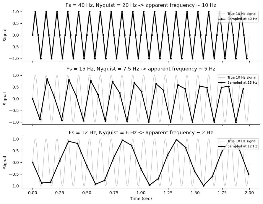
At 40 Hz the samples trace the 10 Hz wave faithfully. At 15 Hz (Nyquist 7.5 Hz), the 10 Hz signal is folded to Hz. At 12 Hz (Nyquist 6 Hz) it appears at Hz — a slow, entirely artifactual oscillation. Let’s confirm the 2 Hz alias in the frequency domain.
fs_new = 12                  # fs_new = sampling rate (Hz); Nyquist = 6 Hz, below the 10 Hz signal
step = round(Fs / fs_new)    # keep every step-th sample of the dense signal
ysub = y[::step]
freqs_sub = np.fft.rfftfreq(len(ysub), d=step / Fs)
mag_sub = np.abs(np.fft.rfft(ysub)) / len(ysub)

plt.figure(figsize=(7, 3.5))
plt.plot(freqs_sub, mag_sub, "k")
plt.axvline(fs_new / 2, color="k", ls=":", label="Nyquist limit (6 Hz)")
plt.xlabel("Frequency (Hz)"); plt.ylabel("Magnitude")
plt.title("Spectrum of the 10 Hz signal sampled at 12 Hz")
plt.legend()
print(f"Spectral peak at {freqs_sub[np.argmax(mag_sub)]:.2f} Hz "
      f"(true signal frequency: {F} Hz)")
Spectral peak at 1.93 Hz (true signal frequency: 10 Hz)
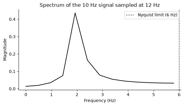
The spectrum of the under-sampled signal peaks near 2 Hz: the 10 Hz signal, 4 Hz above the 6 Hz Nyquist limit, has been reflected to 4 Hz below it. Once data are acquired this way, no analysis can tell the alias apart from a genuine 2 Hz signal.
3. Aliasing a heartbeat at fMRI TRs
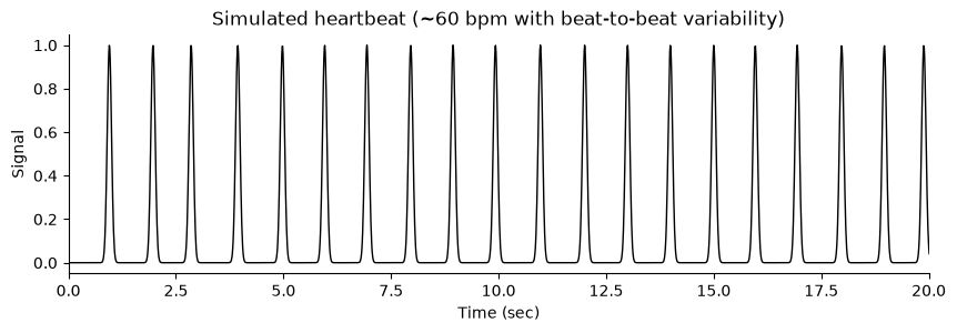
Now the fMRI version of the problem. The cardiac cycle produces a periodic artifact at roughly 1 Hz (60 beats per minute) — far faster than task-related BOLD fluctuations, which typically live below ~0.1 Hz. Whether the heartbeat stays separable from the task depends entirely on the TR. We simulate a spiky heartbeat with realistic beat-to-beat variability, then sample it once per TR, as a scanner would.
fs = 100                          # fs = simulation rate (Hz) — plenty for a ~1 Hz signal
dur = 300                         # dur = duration (s): 5 minutes, a short fMRI run
t = np.arange(0, dur, 1 / fs)

# Beat times: mean interval 1 s (60 bpm) with beat-to-beat jitter
intervals = rng.normal(1.0, 0.06, size=int(dur * 1.2)).clip(0.7, 1.4)   # mean 1 s between beats (60 bpm), sd = 0.06 s jitter
beat_times = np.cumsum(intervals)
beat_times = beat_times[beat_times < dur - 1]

# Each beat: a brief pulse (narrow Gaussian), like a pulse-oximeter trace
heart = np.zeros_like(t)
for bt in beat_times:
    heart += np.exp(-(t - bt) ** 2 / (2 * 0.05 ** 2))

plt.figure(figsize=(10, 2.8))
plt.plot(t, heart, "k", lw=1)
plt.xlim(0, 20); plt.xlabel("Time (sec)"); plt.ylabel("Signal")
plt.title("Simulated heartbeat (~60 bpm with beat-to-beat variability)")
print(f"Mean heart rate: {60 / np.diff(beat_times).mean():.1f} bpm")
Mean heart rate: 59.7 bpm
def sample_at_tr(signal, fs, TR):
    """Sample a densely simulated signal once per TR (volume acquisition)."""
    step = round(TR * fs)
    return signal[::step]

fig, axes = plt.subplots(3, 2, figsize=(11, 9))
for row, TR in zip(axes, (0.5, 1.0, 2.0)):    # TR = time between volumes (s)
    samp = sample_at_tr(heart, fs, TR)
    ts = np.arange(len(samp)) * TR
    nyq = 1 / (2 * TR)

    # Time domain (first 20 s)
    row[0].plot(t, heart, color=".8", lw=1)
    row[0].plot(ts, samp, ".-", color="purple", lw=1.5)
    row[0].set(xlim=(0, 20), xlabel="Time (sec)", ylabel="Signal",
               title=f"TR = {TR} s")

    # Frequency domain
    freqs_s = np.fft.rfftfreq(len(samp), d=TR)
    mag_s = np.abs(np.fft.rfft(samp - samp.mean())) / len(samp)
    row[1].plot(freqs_s, mag_s, color="purple", lw=1)
    row[1].axvline(nyq, color="k", ls=":")
    row[1].axvspan(0.005, 0.1, color="orange", alpha=0.2)
    row[1].set(xlim=(0, 1.1), xlabel="Frequency (Hz)", ylabel="Magnitude",
               title=f"Nyquist = {nyq:g} Hz (dotted); task band shaded")
plt.tight_layout()
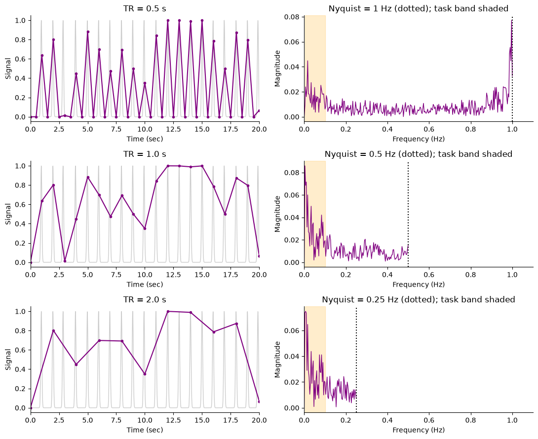
At TR = 0.5 s (Nyquist 1 Hz) most cardiac power sits at or just below 1 Hz — its own neighborhood, far from the shaded task band, where it could be filtered out or modeled. At TR = 1 s and especially TR = 2 s, the cardiac peak has nowhere legal to live: it is folded below the Nyquist limit and smeared across the low frequencies, directly on top of task-related frequencies (roughly 0.005–0.1 Hz). Let’s quantify how much cardiac power lands in the task band at each TR.
print("Fraction of sampled cardiac power falling in the task band (0.005-0.1 Hz):\n")
for TR in (0.4, 0.5, 1.0, 2.0, 3.0):    # TRs from fast multiband to slow standard sampling
    samp = sample_at_tr(heart, fs, TR)
    freqs_s = np.fft.rfftfreq(len(samp), d=TR)
    power = np.abs(np.fft.rfft(samp - samp.mean())) ** 2
    in_band = power[(freqs_s > 0.005) & (freqs_s < 0.1)].sum() / power[1:].sum()
    print(f"  TR = {TR:>3} s  (Nyquist {1/(2*TR):4.2f} Hz):  {100 * in_band:5.1f} %")
Fraction of sampled cardiac power falling in the task band (0.005-0.1 Hz):

  TR = 0.4 s  (Nyquist 1.25 Hz):    1.9 %
  TR = 0.5 s  (Nyquist 1.00 Hz):   22.3 %
  TR = 1.0 s  (Nyquist 0.50 Hz):   59.7 %
  TR = 2.0 s  (Nyquist 0.25 Hz):   68.6 %
  TR = 3.0 s  (Nyquist 0.17 Hz):   70.4 %
A TR of 0.4 s keeps almost all cardiac power out of the task band. Notice the instructive edge case at TR = 0.5 s: its Nyquist limit (1 Hz) sits exactly at the cardiac frequency, so even there a noticeable share of power folds into low frequencies. At TR of 2–3 s a large share of it masquerades as slow “signal”. This is one reason modern accelerated (multiband) protocols push TR below ~0.5 s: physiological noise stays above the task frequencies, where it can be separated from neural signal — a benefit for task analyses and even more so for functional connectivity. (With variable beat-to-beat timing the aliased power is smeared, not a clean single peak — just as in real data.)
4. Is smoothing lossy? Small vs. large activations
Spatial smoothing is the temporal-sampling story’s spatial cousin. Smoothing suppresses noise and absorbs some inter-subject misalignment, but it acts as a matched filter: it is most sensitive to signals at roughly the scale of the kernel, and it attenuates anything smaller. We simulate a 1-D strip of cortex (1 voxel = 1 mm) with two activations of equal amplitude — one narrow (~3.5 mm FWHM, the scale of a small nucleus) and one broad (~19 mm) — plus noise, and smooth with a typical 8 mm FWHM Gaussian kernel.
Inspired by is_smoothing_lossy.m in github
n_vox = 200                                         # n_vox = number of voxels in the 1-D strip
x = np.arange(n_vox)                                # position along the strip: 1 voxel = 1 mm
fwhm2sig = 1 / (2 * np.sqrt(2 * np.log(2)))         # FWHM -> Gaussian sigma

small = 2 * np.exp(-(x - 60) ** 2 / (2 * 1.5 ** 2))    # ~3.5 mm FWHM
large = 2 * np.exp(-(x - 140) ** 2 / (2 * 8 ** 2))     # ~19 mm FWHM
truth = small + large
y = truth + rng.standard_normal(n_vox)                 # noise sd = 1

kernel_fwhm = 8                                        # kernel_fwhm = smoothing kernel FWHM (mm), a typical choice
y_smooth = gaussian_filter1d(y, kernel_fwhm * fwhm2sig)

plt.figure(figsize=(10, 3.8))
plt.plot(x, y, color=".75", lw=1, label="Noisy data")
plt.plot(x, y_smooth, "k", lw=2, label=f"Smoothed ({kernel_fwhm} mm FWHM)")
plt.plot(x, truth, "r--", lw=1.5, label="True signal")
plt.xlabel("Position (mm)"); plt.ylabel("Signal"); plt.legend()
plt.title("Equal-amplitude activations: narrow (left) vs. broad (right)")

print(f"True peak amplitude, both blobs:      2.00")
print(f"Smoothed peak, narrow blob (~3.5 mm): {y_smooth[50:70].max():.2f}")
print(f"Smoothed peak, broad blob (~19 mm):   {y_smooth[130:150].max():.2f}")
True peak amplitude, both blobs:      2.00
Smoothed peak, narrow blob (~3.5 mm): 1.17
Smoothed peak, broad blob (~19 mm):   1.92
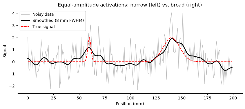
The broad activation survives smoothing nearly intact, while the narrow one — same true amplitude — is flattened to a fraction of its height and could easily fall below a statistical threshold. Smoothing traded away exactly the fine spatial scales we might care most about.
To see the tradeoff more completely, we sweep the activation width and measure two things after smoothing: the recovered peak amplitude (signal attenuation) and the peak z-score (detection sensitivity, averaged over noise realizations). Smoothing reduces noise, so sensitivity can improve even when amplitude shrinks — but only for activations near or above the kernel scale.
blob_fwhms = np.array([2, 3.5, 5, 8, 12, 19, 30])    # activation FWHMs to sweep (mm)
n_sims = 200                                         # n_sims = noise realizations per width; more -> stabler estimates
center = n_vox // 2                                  # place each activation mid-strip

print(f"{'Blob FWHM (mm)':>14} | {'smoothed peak amp':>17} | "
      f"{'peak z (raw)':>12} | {'peak z (smoothed)':>17}")
print("-" * 72)
for bf in blob_fwhms:
    blob = 2 * np.exp(-(x - center) ** 2 / (2 * (bf * fwhm2sig) ** 2))
    amp = gaussian_filter1d(blob, kernel_fwhm * fwhm2sig)[center]

    z_raw, z_sm = [], []
    for _ in range(n_sims):
        noise = rng.standard_normal(n_vox)
        z_raw.append((blob + noise)[center])
        sm = gaussian_filter1d(blob + noise, kernel_fwhm * fwhm2sig)
        sm_noise_sd = gaussian_filter1d(noise, kernel_fwhm * fwhm2sig).std()
        z_sm.append(sm[center] / sm_noise_sd)
    print(f"{bf:>14} | {amp:>17.2f} | {np.mean(z_raw):>12.1f} | {np.mean(z_sm):>17.1f}")
Blob FWHM (mm) | smoothed peak amp | peak z (raw) | peak z (smoothed)
------------------------------------------------------------------------
           2.0 |              0.49 |          2.1 |               1.7
           3.5 |              0.80 |          2.0 |               2.8
           5.0 |              1.06 |          2.1 |               3.9
           8.0 |              1.41 |          2.0 |               5.1
          12.0 |              1.66 |          2.0 |               6.2
          19.0 |              1.84 |          1.9 |               6.7
          30.0 |              1.93 |          2.1 |               7.0
Two lessons sit side by side in this table. Smoothing always attenuates peak amplitude for activations smaller than the kernel — for a 2 mm activation the recovered amplitude is a small fraction of the truth, a partial-volume-like dilution imposed by analysis rather than acquisition. Yet the peak z-score tells a second story: because smoothing suppresses independent voxel noise, detection sensitivity improves for activations at or above the kernel scale, and even modest-sized activations can become easier to detect while being harder to localize precisely. The kernel choice silently decides which spatial scales your study can see — exactly the “effective resolution” argument of Chapter 15.
Wrap-up
The FFT re-expresses a time series as power at each frequency; nothing above the Nyquist limit can be represented.
Signals faster than the Nyquist limit are folded back into low frequencies (aliasing) and become indistinguishable from genuine slow signals.
At common TRs (2–3 s), cardiac signal aliases directly into task frequencies; fast (multiband) sampling keeps it separable.
Spatial smoothing is a matched filter: it boosts detection of activations at its own scale and attenuates smaller ones, lowering the study’s effective spatial resolution.
Back to the chapter: Spatial and Temporal Resolution.