Artifacts and Noise in fMRI
Run this code: ⚡ In-browser lab · Colab · MATLAB Online
Overview
Everything we do in fMRI analysis rests on separating a small signal of interest from a much larger sea of noise. Artifacts are deviations of an image’s spatial pattern or intensity from its true underlying values, along with spurious results produced by confounding processes. They can be introduced — or mitigated — at virtually every stage of acquisition and analysis. Because it is impossible to remove every noise source, what remains is autocorrelated: noise that propagates across time and space, driven by MR physics and BOLD biophysics, hardware instability, head movement, and cardiac and respiratory physiology. This chapter surveys the main artifact types and noise sources; later chapters (17 and 19) cover the preprocessing and modeling steps that address them.
A first family of problems is visible in the images themselves. Susceptibility artifacts arise near air–tissue boundaries (sinuses, ear canals), where local magnetic field inhomogeneities cause geometric distortion (prominent in EPI), blurring (prominent in spiral sequences), and signal dropout. They preferentially affect orbitofrontal cortex, inferior temporal cortex, hypothalamus, and amygdala, and grow stronger at higher field. They are tricky to avoid because sensitivity to field inhomogeneity is also the source of BOLD contrast itself. External electromagnetic sources — RF leakage, vibration, and eddy currents induced in unshielded cables — can inject spikes into k-space that appear as banding across the image, or corrupt images entirely. Other acquisition artifacts include chemical shift (fat and water precess at slightly different frequencies, displacing fat signal in the image), wrap-around ghosting (faint duplicate images along the phase-encode direction when the field of view is too small, or with movement), Gibbs ringing (bright–dark ripples near sharp tissue boundaries caused by truncating the k-space frequency spectrum), and Moiré fringes from field inhomogeneity. The best defense is disarmingly low-tech: look carefully at every participant’s images as they are acquired — quantitative metrics are surprisingly limited by comparison, though they help flag changes in hardware status.
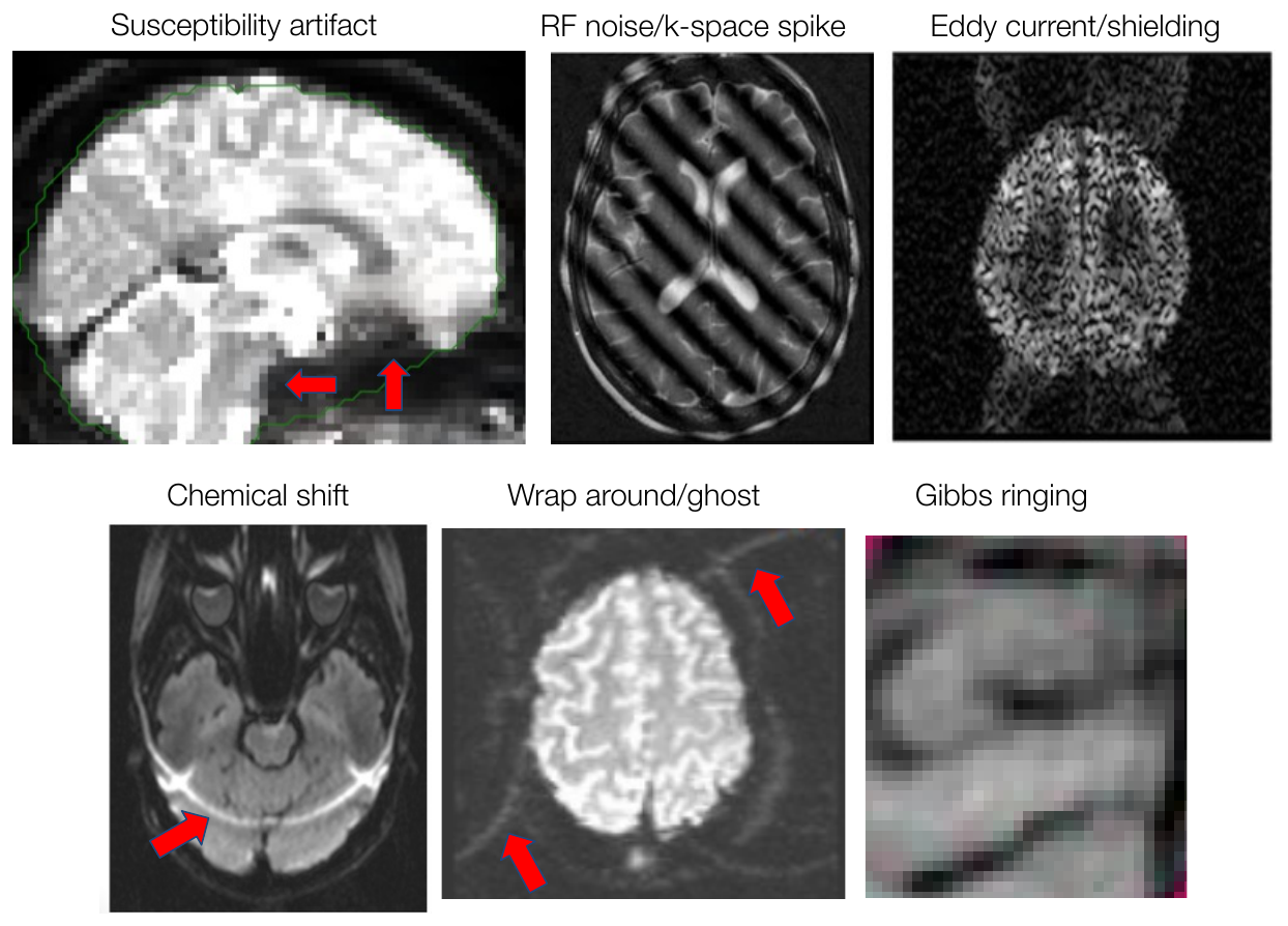
Several common types of image artifacts. These can generally be avoided with appropriate pulse sequences and acquisition parameters, though they are present to some degree in most images. Routine visual inspection matters: new artifacts can signal changes in hardware status and environmental noise. (Figure 16.1 from the book. © the authors and MIT Press; reproduced with permission — not covered by this site’s CC-BY license.)
A second family lives in the time series. fMRI signals drift slowly over a run — visible even in phantoms, so not neural in origin — due to scanner instabilities and slow changes in head position and physiology. To reason about drift, it helps to view signals in the frequency domain: the Fourier transform re-expresses a time series, without loss of information, as a set of sine waves, each with a magnitude (power) and phase. Drift concentrates power at the lowest frequencies, in inverse proportion to frequency — so-called 1/f noise. Because task-related signals often live at nearby low frequencies, drift can mask true effects or masquerade as false ones, and it makes designs in which a process unfolds only once, slowly (a drug high, a developing mood), difficult — though modern, more stable scanners have relaxed this constraint somewhat. Drift is typically removed with a high-pass filter (Chapter 19).
Sampling in time brings its own trap: aliasing. The Nyquist theorem says that capturing a periodic signal requires sampling at least twice its frequency. In fMRI the sampling rate is , so the highest recoverable frequency is the Nyquist limit,
f_Nyquist — highest frequency recoverable from the sampled data (Hz) · F_s — sampling rate, 1/TR (Hz) · TR — repetition time between volumes (s)
where is the highest frequency that can be recovered from the sampled data, the sampling rate, and the repetition time between volumes.
Signals above this limit do not disappear — they are reflected around the Nyquist frequency and reappear as spurious low-frequency fluctuations. With a typical TR of 2 s (Nyquist = 0.25 Hz), a 1 Hz heartbeat is aliased down into the same low-frequency band as the task. Worse, the aliased pattern changes dramatically with small variations in heartbeat timing, so it can be neither cleanly filtered nor easily modeled with covariates.
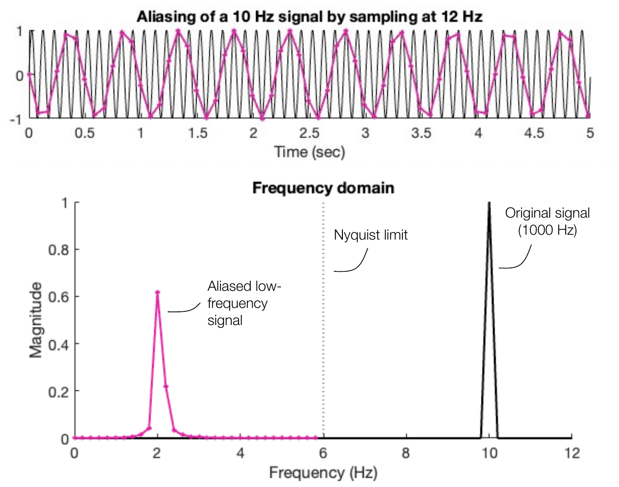
Temporal aliasing caused by under-sampling. A 10 Hz sine wave (black, sampled at 1,000 Hz) is sampled at only 12 Hz (purple). The samples catch different phases of the underlying signal, so it appears to oscillate at a lower frequency. In the frequency domain (bottom), the original signal is reflected around the Nyquist limit (dashed line), reappearing near 2 Hz. (Figure 16.3 from the book. © the authors and MIT Press; reproduced with permission — not covered by this site’s CC-BY license.)
Several noise sources shape the BOLD time series itself. Thermal noise from random electron motion adds independent noise to every voxel; SNR falls with 1 over voxel volume (1 mm isotropic voxels have 27× lower SNR than 3 mm voxels), which is why smoothing and larger voxels help, and why very high resolution only becomes routine at ultra-high field. Transient “spikes” — from gradient imprecision or its interaction with head movement — produce individual images with aberrant intensity. Relatedly, the first few volumes of every run are brighter because T1 contrast has not yet reached steady state; they are routinely discarded (check that the effect has actually dissipated). Head movement produces complex artifacts because the field is not perfectly homogeneous, movement itself distorts the field, and moving tissue is re-excited at irregular intervals, disrupting steady-state saturation (spin-history effects). If movement covaries with the task, it can produce convincing-looking false activations. Physiological noise is pervasive: cardiac pulsation moves tissue and produces inflow effects near vessels; respiration changes the field via thoracic movement, producing spatially distributed phase shifts; and heart rate and breathing depth themselves fluctuate with task demands, placing noise squarely in the frequency band of the HRF.
Transient artifacts can be found with statistical outlier detection applied to each participant’s time series: flagging images with large head movement, high Mahalanobis distance (a multivariate distance from the cloud of other images), and large image-to-image change — the root-mean-square successive difference (RMSSD, called DVARS in the neuroimaging literature). Once identified, outliers are best handled by adding one spike-indicator covariate per bad image to the first-level model, rather than deleting time points — deletion changes the noise structure in ways that complicate filtering and autocorrelation estimation, forces retiming of the design, and can bias sampling if outliers are task-related.
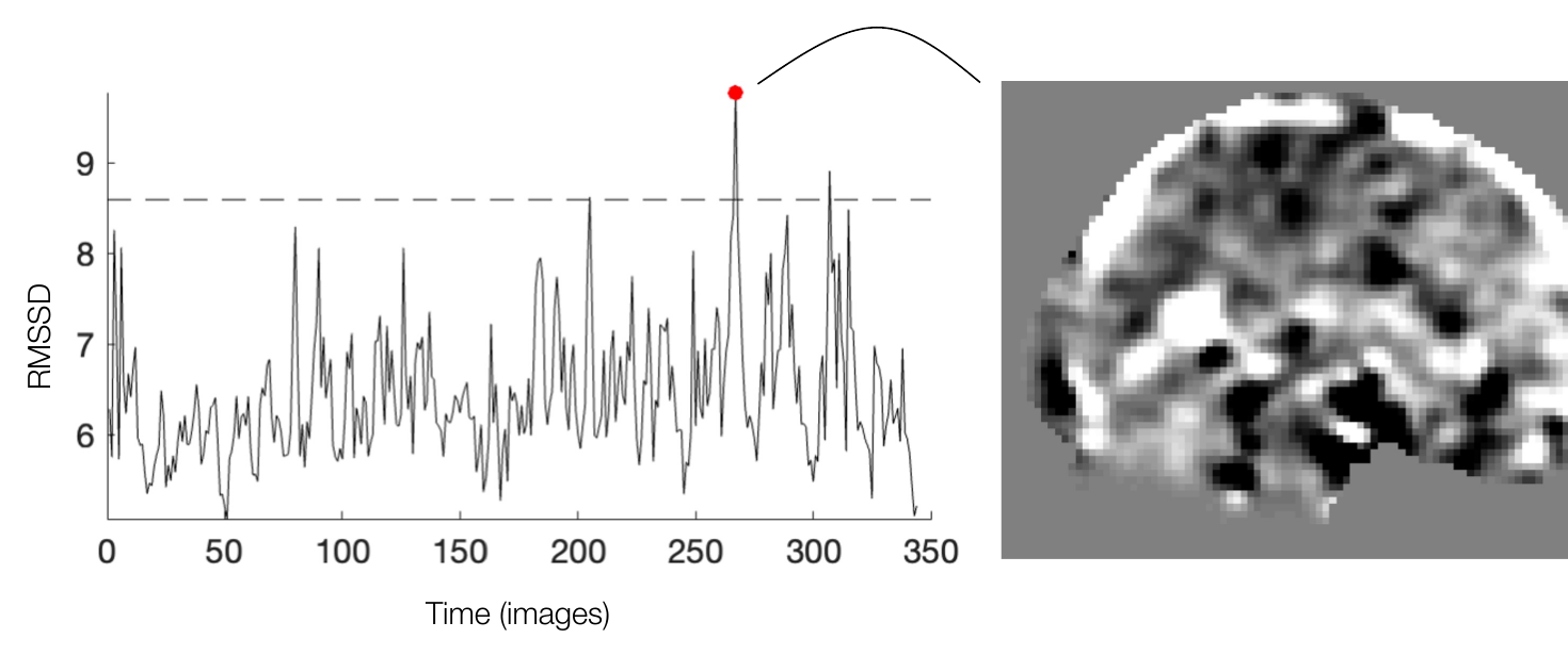
Detecting transient image artifacts with RMSSD (DVARS). BOLD signal changes slowly, but artifacts can be immediate, so the total change from one image to the next is a sensitive diagnostic. The dashed line marks 3 standard deviations above the mean; the flagged image (right) shows a bright rim at the top of the brain and dark areas below — a sudden, spatially broad signal shift. (Figure 16.5 from the book. © the authors and MIT Press; reproduced with permission — not covered by this site’s CC-BY license.)
The residue of all these processes is noise that is correlated across time. Autocorrelation matters because ordinary least squares assumes independent errors: with positively autocorrelated noise, a naive GLM underestimates the uncertainty of its estimates, inflating t-statistics and false positive rates. Chapters 18–19 develop the remedy (generalized least squares with prewhitening); the tutorial below lets you generate the problem — and see the inflation — yourself.
Hands-on tutorial
In this tutorial you will build an fMRI-like time series from its noise ingredients — slow drift, AR(1) autocorrelated noise, transient spikes, and an aliased heartbeat — then detect the outliers and measure what autocorrelation does to naive inference.
Step 1 — Simulate a noisy voxel and flag transient outliers. We assemble a time series from known components, then use successive differences (the single-voxel analog of RMSSD/DVARS) to find the spikes.
% Requires CanlabCore on your MATLAB path (noise_arp)
% Adapted from CANlab tutorials (github.com/canlab)
rng(7);                                          % seed for reproducibility
TR = 2;                                          % TR = repetition time (s)
n  = 240;                                        % n = number of volumes (an 8-min run)
t  = (0:n-1)' * TR;                              % volume acquisition times (s)

drift = 6*cos(2*pi*t/400) + 3*cos(2*pi*t/180);   % slow scanner drift (400-s and 180-s periods)
phi = 0.5;                                       % AR(1) coefficient: each error keeps half the last
ar  = noise_arp(n, phi);                         % AR(1) autocorrelated noise
y   = 100 + drift + ar;                          % baseline of 100 + drift + noise
y([61 62 151]) = y([61 62 151]) + [18 -12 15]';  % transient spikes in 3 volumes

rmssd = [NaN; abs(diff(y))];                     % successive differences (single-voxel DVARS)
z = (rmssd - mean(rmssd, 'omitnan')) ./ std(rmssd, 'omitnan');  % z-score the differences
wh = find(z > 3)                                 % flagged volumes: change > 3 SD above the mean

figure; plot(t, y, 'k-'); hold on;               % time series with flagged volumes marked
plot(t(wh), y(wh), 'ro', 'MarkerFaceColor', 'r');
xlabel('Time (s)'); ylabel('Signal (a.u.)');
import numpy as np
import matplotlib.pyplot as plt
rng = np.random.default_rng(7) # seed for reproducibility
TR, n = 2.0, 240 # TR = repetition time (s); n = volumes (8-min run)
t = np.arange(n) * TR # volume acquisition times (s)
drift = 6*np.cos(2*np.pi*t/400) + 3*np.cos(2*np.pi*t/180) # slow scanner drift
eta, ar = rng.standard_normal(n), np.zeros(n) # eta = white noise; ar = AR(1) noise
for i in range(1, n):
ar[i] = 0.5 * ar[i-1] + eta[i] # phi = 0.5: each error keeps half the last
y = 100 + drift + ar # baseline of 100 + drift + noise
y[[60, 61, 150]] += [18, -12, 15] # transient spikes in 3 volumes
rmssd = np.abs(np.diff(y)) # successive differences (single-voxel DVARS)
z = (rmssd - rmssd.mean()) / rmssd.std() # z-score the differences
flagged = np.where(z > 3)[0] + 1 # flagged volumes: change > 3 SD above the mean
print("Flagged volumes:", flagged)
plt.figure(figsize=(8, 3)) # time series with flagged volumes marked
plt.plot(t, y, "k", lw=0.8, label="voxel time series")
plt.plot(t[flagged], y[flagged], "ro", ms=5, label="flagged volumes")
plt.xlabel("Time (s)"); plt.ylabel("Signal (a.u.)"); plt.legend(fontsize=8)Example output:
Flagged volumes: [ 60 61 62 150 151]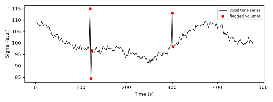
The simulated voxel with its three inserted spikes. The successive-difference test flags the spike volumes — and the volumes just after them, because a spike produces a large change both into and out of the artifact. In practice, adjacent flagged volumes are all treated as outliers.
Step 2 — See autocorrelation break naive OLS. We fit a blocked task regressor to pure AR(1) noise — no signal at all — thousands of times. With independent noise, about 5% of tests should be “significant” at p < .05. Watch what actually happens.
X = [double(sin(2*pi*t/80) > 0), ones(n, 1)];    % 40-s on/off blocks + intercept
c = inv(X'*X);                                   % (X'X)^-1, used for standard errors
nfp = 0;                                         % nfp = false positive counter
nsim = 2000;                                     % nsim = number of null simulations
for i = 1:nsim
    e = noise_arp(n, phi);                       % null data: AR(1) noise only, no signal
    b = X \ e;  r = e - X*b;                     % OLS fit and residuals
    se = sqrt((r'*r)/(n-2) * c(1,1));            % naive OLS standard error
    nfp = nfp + (abs(b(1)/se) > tinv(.975, n-2));  % count |t| beyond the two-sided .05 cutoff
end
nfp / nsim     % false positive rate: several times the nominal 0.05
from scipy import stats
X = np.c_[(np.sin(2*np.pi*t/80) > 0).astype(float), np.ones(n)] # 40-s blocks + intercept
c = np.linalg.inv(X.T @ X) # (X'X)^-1, used for standard errors
tcrit, nfp, nsim = stats.t.ppf(0.975, n - 2), 0, 2000 # .05 critical value; counter; number of null simulations
for _ in range(nsim):
eta, e = rng.standard_normal(n), np.zeros(n) # null data: AR(1) noise only, no signal
for i in range(1, n):
e[i] = 0.5 * e[i-1] + eta[i] # phi = 0.5, as in Step 1
b = np.linalg.lstsq(X, e, rcond=None)[0] # OLS fit
r = e - X @ b # residuals
se = np.sqrt(r @ r / (n - 2) * c[0, 0]) # naive OLS standard error
nfp += abs(b[0] / se) > tcrit # count |t| beyond the two-sided .05 cutoff
print("False positive rate:", nfp / nsim) # several times the nominal 0.05Example output:
False positive rate: 0.2355Nearly five times the nominal 0.05 — every one of those a “significant activation” in data containing no signal at all.
The full labs go further: they visualize each noise component and its power spectrum, demonstrate temporal aliasing with a jittered heartbeat sampled at the TR, detect outliers in a multi-voxel dataset with both RMSSD/DVARS and Mahalanobis distance, build spike regressors, and show that prewhitening restores valid false positive rates.
Open the full Python lab notebook → or download the MATLAB live script, which mirrors it using CANlab tools.


Thought questions
Susceptibility artifacts arise from the very field-inhomogeneity sensitivity that makes BOLD imaging possible, and they worsen at higher field strength. If you were designing a study of the orbitofrontal cortex and amygdala, how would this shape your choices about field strength, voxel size, pulse sequence, and how you interpret “no activation” in those regions?
A 1 Hz heartbeat sampled at TR = 2 s is aliased into the low-frequency band occupied by the task — and the aliased pattern shifts unpredictably with small changes in beat timing. Why does this combination defeat both high-pass filtering and covariate modeling? What acquisition or physiological-monitoring strategies could restore your ability to separate cardiac noise from signal?
The chapter recommends modeling outlier images with spike covariates rather than deleting them from the time series. Construct a concrete scenario in which deleting task-correlated outliers (say, motion during painful stimuli) biases the resulting activation estimates, and explain the direction of the bias.
Head movement affects the signal through several distinct mechanisms — field inhomogeneity sampled at new positions, movement-induced field distortion, and spin-history effects. Why does this multiplicity imply that rigid-body realignment (Chapter 17) cannot fully correct movement artifacts, even in principle?
Many labs rely on automated QC metrics; the book argues visual inspection is still indispensable. Where do you think each approach is strong and weak, and what would a QC protocol that combines them look like for a 200-participant study?
Quiz yourself
Q1. What is an artifact in fMRI, and name three broad categories discussed in this chapter.
Answer: An artifact is a deviation of an image’s spatial pattern or intensity from its true underlying values (or a spurious result from a confounding process). Categories include susceptibility artifacts, artifacts from external electromagnetic sources (RF spikes, vibration, eddy currents), and aliasing/ghosting-type artifacts such as chemical shift, wrap-around ghosts, Gibbs ringing, and Moiré fringes.
Q2. Which brain regions are most affected by susceptibility artifacts, and why are these artifacts hard to eliminate?
Answer: Regions near air–tissue boundaries at the base of the brain: orbitofrontal cortex, inferior temporal cortex, hypothalamus, and amygdala. They are hard to eliminate because the sensitivity to magnetic field inhomogeneity that produces them is the same sensitivity that produces the BOLD signal itself — and they grow stronger at higher field.
Q3. What is the Nyquist limit for an fMRI acquisition with TR = 2 s, and what happens to a 1 Hz cardiac signal in such data?
Answer: The Nyquist limit is Hz. A 1 Hz heartbeat exceeds it and is aliased — reflected around the Nyquist frequency — reappearing as spurious low-frequency fluctuations that overlap the task frequency band.
Q4. How does thermal noise scale with voxel size, and what practical steps reduce its impact?
Answer: SNR decreases as 1 over the voxel volume — 1 mm isotropic voxels have 27 times lower SNR than 3 mm voxels. Because thermal noise is spatially independent, acquiring larger voxels or averaging across voxels (spatial smoothing) reduces its impact; at 3T it is usually not limiting until voxels are around 1.5 mm or smaller.
Q5. What is RMSSD/DVARS, and why is it a good detector of transient artifacts?
Answer: RMSSD (root-mean-square successive difference, called DVARS in neuroimaging) measures the total change in the image from one time point to the next. Because true BOLD signal changes slowly while artifacts can be immediate, a large image-to-image change (e.g., beyond 3 SD of the mean RMSSD) is a sensitive flag for transient outliers and sudden shifts.
Q6. Why is modeling outlier images with covariates preferred over deleting them from the time series?
Answer: Deletion (1) changes the noise properties in ways not easily accounted for in high-pass filtering and autocorrelation estimation, (2) requires adjusting the experimental timing, and (3) can introduce sampling bias if outliers are task-related (e.g., motion during certain conditions), leading to incorrect inference. A spike-indicator covariate removes each bad image’s influence while preserving the time series structure.
Q7. Name the three reasons head movement corrupts the fMRI signal beyond simple spatial misalignment.
Answer: (1) The magnetic field is not perfectly homogeneous, so a voxel samples different field strengths as the head moves; (2) head movement itself induces distortions in the field; and (3) spin-history effects — moving tissue is re-excited at irregular intervals, disrupting steady-state saturation and producing signal changes across the image.
Q8. Why does autocorrelated noise inflate false positive rates in a naive OLS analysis?
Answer: OLS standard errors assume independent errors. Positively autocorrelated noise contains fewer independent observations than the number of time points, so the true variability of the estimates is larger than OLS computes. The underestimated standard errors inflate t-statistics, making P values too liberal — the remedy is generalized least squares with prewhitening (Chapters 18–19).
 The book: Elements of Functional Magnetic Resonance Imaging — Wager & Lindquist, MIT Press