GLM Design Specification
Run this code: ⚡ In-browser lab · Colab · MATLAB Online
Overview
Chapter 18 gave us the machinery of the GLM: convolve stimulus functions with an HRF, assemble a design matrix , and estimate by least squares. This chapter is about the craft of specifying that model. The same experiment can be modeled many ways — brief events or sustained epochs, fixed or variable durations, with or without trial-by-trial modulators, with more or fewer nuisance covariates — and these choices determine what your betas mean, how much power you have, and whether artifacts masquerade as brain activity. The same GLM framework also serves resting-state fMRI, where it is used as a preprocessing step to remove drift and nuisance signals before connectivity analysis.
Choosing task regressors. The starting choice is how to represent each condition’s neural activity. Brief stimuli are usually modeled as events (impulses or short boxcars), sustained states as epochs (long boxcars); after HRF convolution these produce very different predictor shapes. When the duration of a process varies from trial to trial — reaction time is the classic example — you can build variable-duration regressors in which each trial’s boxcar lasts as long as the process it models. A related tool is the parametric modulator: a regressor whose amplitude scales with a trial-by-trial variable (pain ratings, stimulus value, RT). The modulated regressor is entered alongside the unmodulated (“average response”) regressor, so that the average beta captures the response to a typical event and the modulator beta captures how the response scales with the variable. Because a modulated regressor is built from the same onsets as its parent, the two are often substantially correlated — mean-centering the modulator values helps, and software such as SPM additionally orthogonalizes the modulator with respect to the average regressor. As we will see below, orthogonalization has consequences that are widely misunderstood.
High-pass filtering. fMRI signal drifts slowly over time even without a task, due to scanner instabilities, head motion, and aliased physiological noise, so most noise power lives at the lowest temporal frequencies. High-pass filtering passes fluctuations faster than a cutoff frequency and attenuates slower ones. It can be applied by pre-filtering each voxel’s time series during preprocessing (as with SPM’s discrete cosine transform filter) — in which case the design matrix must be filtered the same way — or by adding drift regressors inside the GLM: a set of low-frequency cosines (or polynomials or splines) whose frequencies span everything below the cutoff. Both routes remove the same variance; the within-GLM route also makes the accounting explicit, with the drift columns absorbing the slow noise while the task columns explain the task.
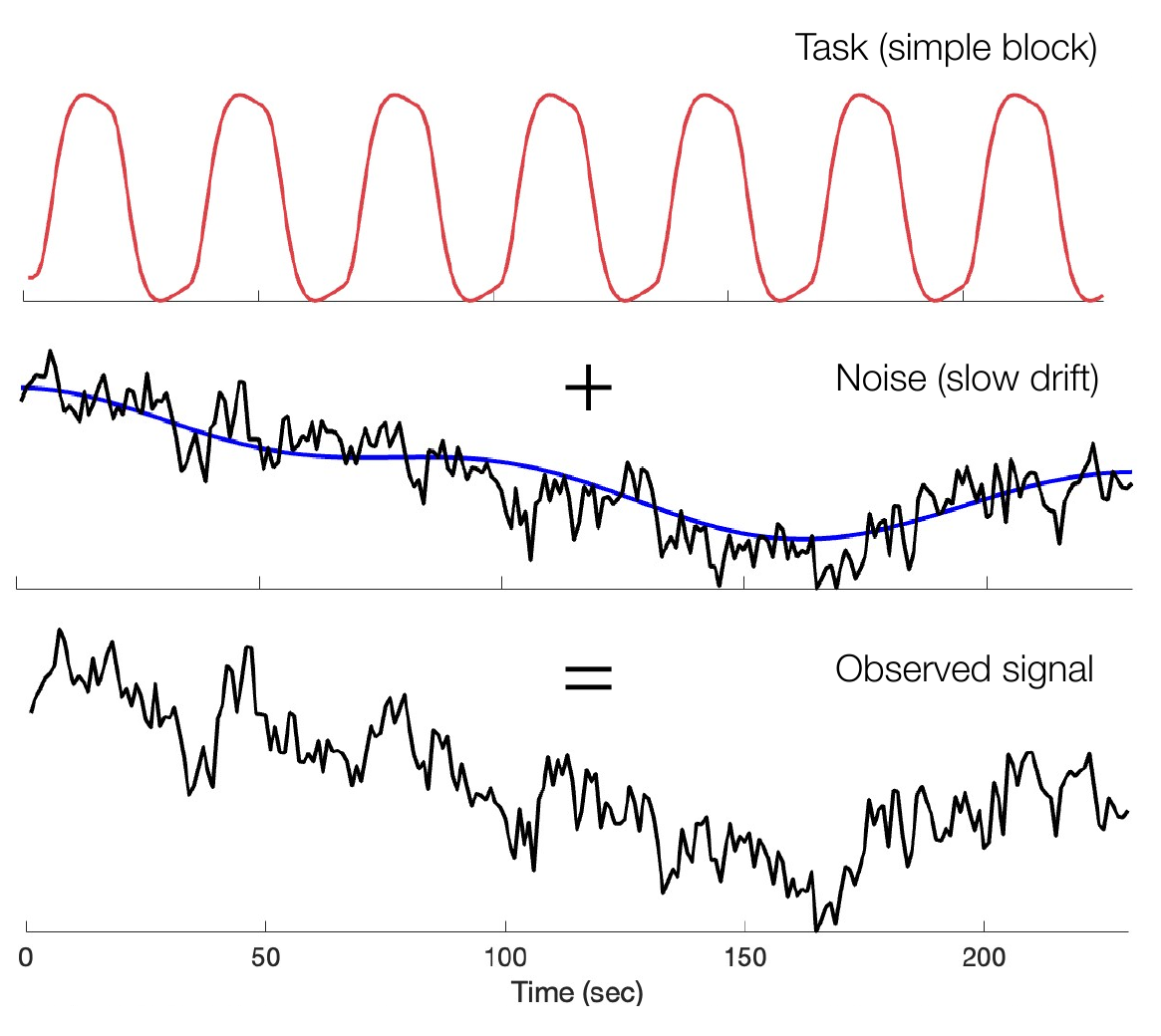
Slow drift in task fMRI. The observed signal (bottom) is the sum of a task-related effect (top, a simple block design alternating every 16 s) and noise dominated by slow drift (middle, blue). In the frequency domain the task oscillates at 0.0312 Hz, well above a typical high-pass cutoff of 1/128 s (0.0078 Hz), so filtering removes much of the drift while sparing the task signal. (Figure 19.1 from the book. © the authors and MIT Press; reproduced with permission — not covered by this site’s CC-BY license.)
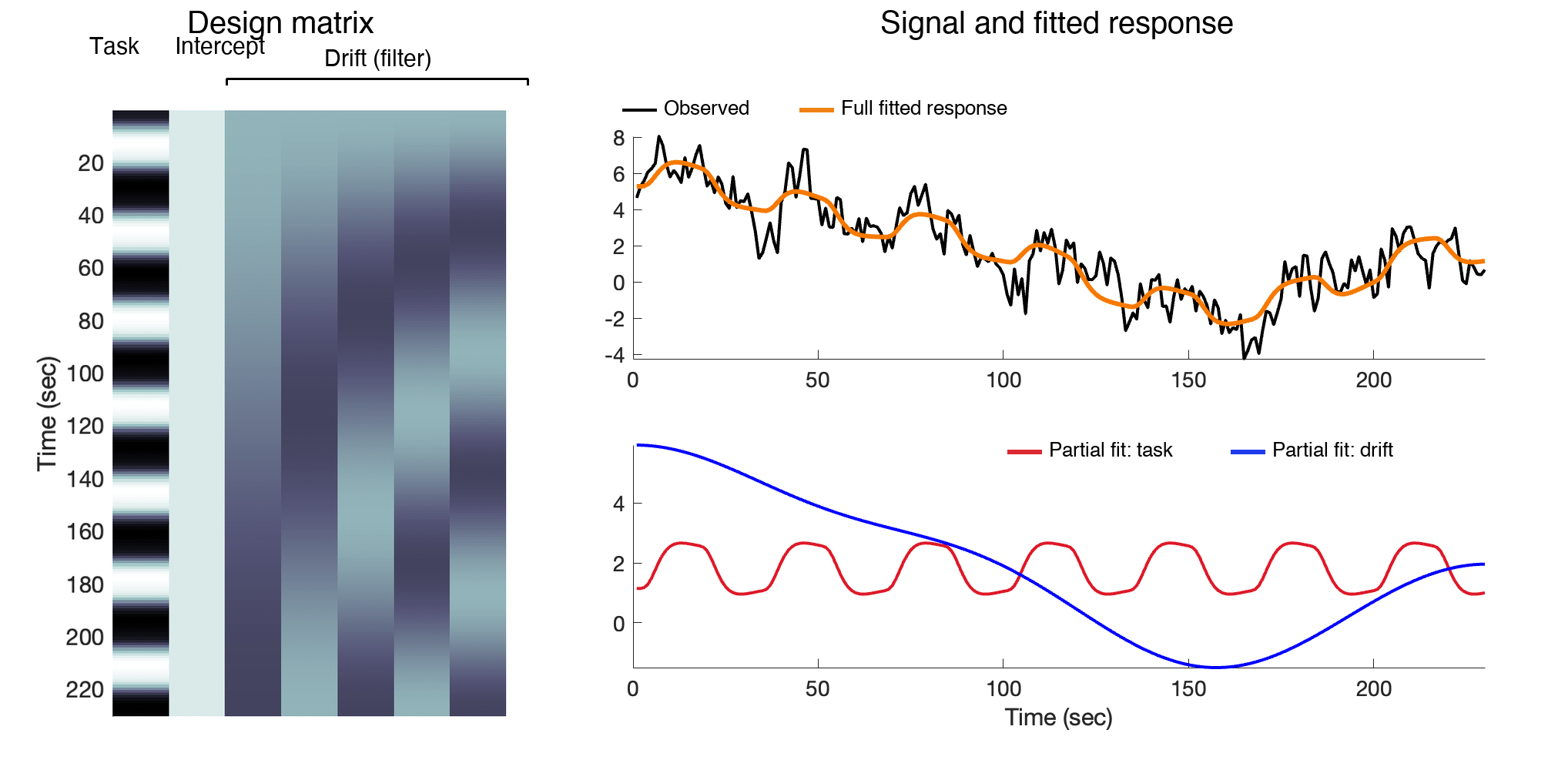
Filtering inside the GLM with nuisance covariates. Left: a design matrix with a task regressor, an intercept, and a set of low-frequency cosine functions. Right: the observed data (black) with the full fitted response (orange), and the contributions of sub-partitions of — the cosine set captures the slow drift (blue) while the task regressor captures the task response after controlling for drift (red). (Figure 19.2 from the book. © the authors and MIT Press; reproduced with permission — not covered by this site’s CC-BY license.)
Choosing the cutoff is a design decision. The task frequencies must stay above the cutoff: for simple block designs, a rule of thumb is a cutoff period of roughly twice the task period. The SPM default is 1/128 s (0.0078 Hz), and resting-state pipelines commonly use 0.01 Hz. Event-related designs are trickier because their variance is spread across frequencies — and what matters is the variance of the contrasts you care about, not just individual regressors. In the example below, an 80 s filter barely touches each regressor but removes about 12% of the A − B contrast variance. Filtering buys power only when it removes more noise than task-related signal.
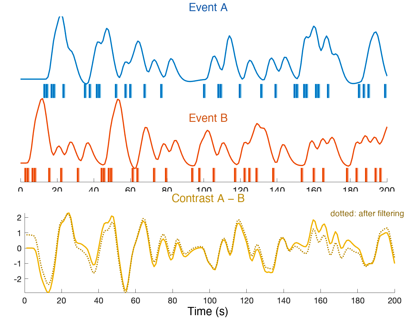
Filtering a randomized event-related design. Predicted activity for event types A (blue) and B (red), and for the contrast A − B (gold). A high-pass filter of 80 s (0.0125 Hz) leaves the individual regressors largely intact but removes about 12% of the contrast variance — the dotted line shows the contrast after filtering. Deviations reflect lost task-related signal. (Figure 19.3 from the book. © the authors and MIT Press; reproduced with permission — not covered by this site’s CC-BY license.)
Nuisance covariates. Nuisance covariates model known sources of variability unrelated to the hypotheses: slow drift, head motion, and physiological artifacts. The most common are the six realignment parameters (three translations, three rotations), often expanded with their squares, derivatives, and squared derivatives into 24 motion covariates per run. High-motion or artifact-contaminated volumes can be handled with spike regression — one indicator regressor per bad image (identified by framewise displacement, DVARS, or Mahalanobis distance) — which absorbs all variance from that volume; spike regression is preferred to scrubbing because it preserves the temporal structure needed for valid variances and P values. Physiological noise can be modeled from measured cardiac and respiratory signals (e.g., RETROICOR, RVHRCOR), or approximated by signals from tissue compartments assumed to contain no signal of interest — mean or principal-component (CompCor) time courses from eroded white matter and CSF masks. None of these is guaranteed to remove only noise: WM/CSF signals can contain real task-related signal, physiology differs systematically across groups, and global signal regression can induce spurious negative correlations through collider bias. Less aggressive strategies with fewer regressors are often preferred, and drift removal and nuisance regression must be done in one step (or later regressors filtered to match), or nuisance regression can reintroduce the low-frequency signals filtering removed.
Collinearity and the VIF. Every regressor you add competes with the others to explain variance. When columns of are correlated, parameter estimates become unstable, their variances grow, and the estimates themselves become (negatively) correlated. Pairwise correlations do not tell the whole story — what matters is whether one predictor can be expressed as a linear combination of all the others. The variance inflation factor for predictor is
VIFᵢ — variance inflation factor for predictor i · Rᵢ² — proportion of variance in predictor i explained by all the other predictors
where is the variance inflation factor for predictor and is the coefficient of determination (proportion of variance explained) from regressing predictor on all the other predictors in the design matrix.
A VIF of 1 is ideal; a VIF of 2 means the variance of has doubled relative to an orthogonal design. In fMRI, VIFs above about 4 warrant serious attention, and above 8 power suffers dramatically and effects are easily misattributed. We care mainly about VIFs for task regressors and contrasts — correlations among nuisance regressors are harmless, but nuisance–task correlations inflate task VIFs, and comparing task VIFs with and without the nuisance set is a good diagnostic. When collinearity is high, honest options are to simplify the design (average correlated variables, pick one, or extract factors) or to use penalized regression (ridge, lasso), accepting bias to reduce variance.
The orthogonalization pitfall. It is tempting to “fix” a correlated pair by orthogonalizing one regressor with respect to the other. But orthogonalization does not create information — it reassigns the shared variance. If is orthogonalized with respect to , the estimate for the orthogonalized is unchanged from its partial estimate in the original model; what changes is , which now absorbs all the variance the two regressors shared. This is appropriate for a parametric modulator, where the average regressor should get credit for the average response. It is inappropriate when the shared variance is genuinely ambiguous — for example, orthogonalizing an RT regressor with respect to condition regressors renders it useless for controlling RT confounds across conditions. Orthogonalize only when you have a principled reason to assign the shared variance to one regressor.
Autocorrelated errors. Finally, the GLM’s independence assumption fails for fMRI: errors are autocorrelated (“colored noise”), partly because omitted covariates have effects that persist across time points. With positive autocorrelation, OLS standard errors are too small and first-level false positive rates too high. The remedy has two parts: model known noise sources (filtering and nuisance regression, above), and model the remaining error covariance with a time-series model. The workhorse is the autoregressive process; an AR(1) error evolves as
εₜ — model error at time t · φ — autoregressive coefficient (|φ| < 1) · zₜ — new white-noise innovation at time t · h — lag (number of time points between two errors)
where is the model error at time point , is the autoregressive coefficient governing how strongly error persists from one time point to the next (), is the new white-noise innovation entering at time , and is the lag (number of time points) separating two errors.
so correlation decays exponentially with lag . Estimated AR parameters define an error covariance matrix , and prewhitening with plus generalized least squares yields valid inference, iterating between estimates of and and adjusting the effective degrees of freedom. Software differs: SPM pools a global AR(1) (or the more flexible FAST dictionary), FSL smooths a regularized unstructured estimate, and AFNI fits a voxel-wise ARMA(1,1). Comparisons favor local, moderate-order models — current recommendations for fast-TR data are higher-order AR models (e.g., AR(4)) combined with physiological noise removal.
Hands-on tutorial
In this tutorial you will make the modeling choices above concrete: build a design with a parametric modulator, measure its collinearity with the average-response regressor, see exactly what orthogonalization does to the betas, and then add a cosine drift set and motion covariates and check their impact on task VIFs.
Step 1 — Parametric modulation and orthogonalization. We model one event type plus a trial-by-trial modulator (e.g., pain ratings), quantify the collinearity between the average and modulated regressors, and compare fits with the raw vs. orthogonalized modulator.
% Requires CanlabCore + SPM12; adapted from CANlab tutorials (github.com/canlab)
TR = 2;                                     % repetition time (s)
runlen = 360;                               % run length (s) -> 180 volumes
ons = {(10:24:340)'};                       % one event type: 14 onsets, every 24 s
ratings = [3 5 2 7 4 6 1 8 5 3 7 2 6 4]';  % trial-by-trial modulator (e.g., pain ratings)

% 'parametric_standard' adds a mean-centered modulator regressor
% Columns: [Avg response, Modulator, intercept]
X = onsets2fmridesign(ons, TR, runlen, 'hrf', 'parametric_standard', {ratings});

corr(X(:, 1), X(:, 2))                      % collinearity of avg & modulator
getvif(X(:, 1:2), false, 'plot')            % variance inflation factors

% Manual orthogonalization of any regressor: resid() removes what x1 explains
% x2_orth = resid(x1, x2, true);
import numpy as np, pandas as pd
from nilearn.glm.first_level import make_first_level_design_matrix
t_r, n_scans = 2.0, 180 # t_r = repetition time (s); n_scans = # volumes
frame_times = np.arange(n_scans) * t_r # volume acquisition times (s)
onsets = np.arange(10, 341, 24.0) # 14 event onsets, every 24 s
ratings = np.array([3, 5, 2, 7, 4, 6, 1, 8, 5, 3, 7, 2, 6, 4.0]) # 1 rating/trial
# Average-response rows carry modulation 1; modulator rows the CENTERED ratings
ev = pd.DataFrame({"onset": onsets, "duration": 1.0, # 1-s events
"trial_type": "pain", "modulation": 1.0})
mod = ev.assign(trial_type="pain_x_rating",
modulation=ratings - ratings.mean()) # mean-center!
X = make_first_level_design_matrix(frame_times,
pd.concat([ev, mod], ignore_index=True),
hrf_model="spm", # canonical SPM HRF
drift_model=None) # no drift terms yet (Step 2)
r = np.corrcoef(X["pain"], X["pain_x_rating"])[0, 1] # collinearity
vif = 1 / (1 - r**2) # VIF for 2 regressors
print(f"corr = {r:.2f}, VIF = {vif:.2f}")
# Orthogonalize the modulator with respect to the average regressor
x1, x2 = X["pain"].to_numpy(), X["pain_x_rating"].to_numpy()
x2_orth = x2 - x1 * (x1 @ x2) / (x1 @ x1) # projection residualExample output:
corr = -0.00, VIF = 1.00With the mean-centered modulator the two regressors are essentially uncorrelated — there is no collinearity left to worry about (compare the raw modulator in the lab, where and the VIF is near 5).
Fit both versions to the same simulated data and compare: the modulator’s beta is identical with or without orthogonalization — only the average regressor’s beta changes, absorbing the shared variance. In the lab, with a raw (uncentered) modulator correlated at with the average regressor, that shift is dramatic — the average beta goes from -1.19 to 0.97 (true value 1.0) — while with a mean-centered modulator there is almost no shared variance left to reassign. Centering, not orthogonalization, is the real fix.
Step 2 — Drift and motion covariates. We add a cosine drift set (high-pass filtering inside the GLM) and six motion covariates, then compare task-regressor VIFs with and without the nuisance set.
n = runlen / TR;                            % number of volumes (180)
k = fix(2 * runlen / 128 + 1);              % # cosine functions for a 128-s cutoff
drift = spm_dctmtx(n, k);                   % DCT drift basis (col 1 = constant)
mot = cumsum(randn(n, 6) * 0.02);           % 6 realignment params, simulated as random walks

Xfull = [X(:, 1:2) mot drift];              % task + motion + drift + constant

vif_task_alone = getvif(X(:, 1:2));         % task VIFs, task-only design
vif_task_full  = getvif(Xfull);             % task VIFs with the full nuisance set
disp([vif_task_alone(1:2); vif_task_full(1:2)])  % compare task VIFs
rng = np.random.default_rng(7) # seeded RNG so results reproduce exactly
mot = np.cumsum(rng.standard_normal((n_scans, 6)) * 0.02,
axis=0) # 6 motion params, simulated as slow random walks
# Cosine drift set for a 128-s cutoff, plus motion, inside the GLM
Xfull = make_first_level_design_matrix(
frame_times, pd.concat([ev, mod], ignore_index=True), hrf_model="spm",
drift_model="cosine", high_pass=1/128, # cutoff frequency (Hz) = 1/(128 s)
add_regs=mot, add_reg_names=[f"mot{i}" for i in range(6)])
def vifs(X): # VIF for each column, given the others (excluding constant)
Xz = X.drop(columns="constant")
Xc = (Xz - Xz.mean()) / Xz.std()
return pd.Series(np.diag(np.linalg.inv(np.corrcoef(Xc.T))), Xz.columns)
print(vifs(Xfull)[["pain", "pain_x_rating"]]) # task VIFs with nuisance setExample output:
pain             1.096307
pain_x_rating    1.156518
dtype: float64
If task VIFs stay near 1, the nuisance set is cheap insurance; if they jump, task and nuisance variance are confounded, and significance will (rightly) drop.
Open the full Python lab notebook → or download the MATLAB live script, which mirrors it using CANlab tools — including variable-duration regressors, the orthogonalization demonstration, spike regressors, and drift-filtering effects on contrasts.


Thought questions
Your design has two block conditions that alternate slowly, completing a full cycle every 150 seconds. Your colleague applies the SPM default high-pass cutoff of 128 s. What will happen to your task effects, and how would you diagnose the problem before ever looking at brain data?
Reaction time correlates with task difficulty in nearly every cognitive experiment. Compare three modeling strategies — ignoring RT, adding RT as an orthogonalized parametric modulator, and adding a variable-duration RT regressor without orthogonalization. For each, what question can you still answer, and what confound remains?
A reviewer asks you to add 24 motion covariates, CompCor components, and spike regressors to a design with 160 volumes. Using the concepts of error degrees of freedom, task VIFs, and shared task–nuisance variance, make the case for and against complying in full.
Global signal regression reduces the correlation between head motion and connectivity estimates but induces negative correlations via collider bias. If two labs analyze the same resting-state data with and without GSR and reach different conclusions about a clinical group difference, is either analysis “wrong”? What would you want to see reported?
Autocorrelation modeling happens at the first level, yet group inference (Chapter 21) is valid even if it is ignored. Why, then, do modern pipelines still invest in voxel-wise AR/ARMA models — what is gained, and for which analyses is it indispensable?
Quiz yourself
Q1. Why is high-pass filtering routinely applied to fMRI time series?
Answer: fMRI signal drifts slowly over time due to scanner instabilities, head motion, and aliased physiological noise, so most noise power is concentrated at the lowest frequencies. A high-pass filter removes these slow fluctuations while passing the faster task-related signals.
Q2. What are the two ways to implement high-pass filtering, and what must you remember if you pre-filter the data?
Answer: (1) Pre-filter each voxel’s time series during preprocessing (e.g., SPM’s DCT filter), or (2) include low-frequency drift regressors (cosines, polynomials, splines) as columns of the GLM design matrix. If you pre-filter the data, you must apply the same filter to the design matrix (and to any nuisance regressors added later) — otherwise regression can reintroduce the removed low-frequency signals.
Q3. How should you choose the high-pass cutoff for a simple block design, and why is the choice harder for event-related designs?
Answer: For block designs, a rule of thumb is a cutoff period of about twice the task period, so the task frequency stays above the cutoff. Event-related designs spread their variance across many frequencies, so any cutoff removes some task and contrast variance; you must check how much contrast variance the filter removes, because filtering only helps if it removes more noise than signal.
Q4. What is spike regression, and why is it preferred to scrubbing (deleting volumes)?
Answer: Spike regression adds one indicator regressor per artifact-contaminated volume (value 1 at that volume, 0 elsewhere), which absorbs all of that volume’s variance so it cannot bias other estimates. It is preferred to scrubbing because it preserves the natural temporal structure of the time series, keeping autocorrelation modeling, variance estimates, and P values valid.
Q5. Define the variance inflation factor and give rough guidelines for interpreting its values in fMRI.
Answer: , where is from regressing predictor on all other predictors. VIF = 1 is ideal (no collinearity); VIF = 2 means the variance of that beta has doubled. In fMRI, VIFs above about 4 warrant serious concern and mitigation, and values of 8 or more cause severe power loss and potential misattribution of effects.
Q6. You orthogonalize a parametric modulator with respect to the average task regressor. Whose beta estimate changes, and whose stays the same?
Answer: The modulator’s beta is unchanged — it already equals the partial (unique) effect from the non-orthogonalized model. The average regressor’s beta changes: it absorbs all the variance the two regressors shared. Orthogonalization reassigns shared variance; it does not create new information.
Q7. Why do correlations among nuisance regressors not matter, while correlations between nuisance and task regressors do?
Answer: Nuisance regressors are included only to remove variance jointly — we never interpret their individual betas, so their mutual collinearity is irrelevant. But nuisance–task correlations inflate the variance (and VIFs) of the task betas, reducing significance — appropriately so, because it becomes unclear whether task or nuisance sources drive the response. Comparing task VIFs with and without the nuisance set diagnoses this.
Q8. What happens to first-level inference if positive error autocorrelation is ignored, and what is the standard fix?
Answer: Standard errors are underestimated, t-statistics are inflated, and false positive rates exceed the nominal level. The fix is to model the error covariance with a time-series model (commonly AR(p) or ARMA(1,1)), prewhiten the data and design with , estimate by generalized least squares iterating between and , and adjust the error degrees of freedom accordingly.
 The book: Elements of Functional Magnetic Resonance Imaging — Wager & Lindquist, MIT Press