Localizing and Interpreting Results
Run this code: ⚡ In-browser lab · Colab · MATLAB Online
Overview
Group analyses (and sometimes single-subject analyses) yield thresholded maps of brain areas significantly related to a stimulus type, task, or behavior. Interpreting those maps — turning colored blobs into claims about the brain — is one of the most important and challenging parts of functional neuroimaging. Deriving meaning is a cumulative enterprise across many studies: what it means to activate a particular patch of dorsolateral prefrontal cortex (dlPFC) during emotion regulation depends on which other tasks engage that patch, which networks it participates in, and what lesions and stimulation there do. Localizing findings against established brain atlases is the key step that makes this integration possible.
An atlas is a standard brain labeled with regions and the boundaries between them, based on histology, structural landmarks, patterns of structural and functional connectivity, neurochemistry, prior neuroimaging findings, and more. Atlases play a role similar to the definition of genes in genetics: they provide uniform labels and precisely defined units of analysis, so that findings from different studies can be compared directly. Without one, two studies may both report “dlPFC” activation while their clusters do not even overlap. Atlases can be built from a single brain or from group averages of co-registered brains, and they can supply either fixed labels (each voxel assigned to one structure) or probabilistic maps (the likelihood that each voxel belongs to each structure, estimated from a set of labeled brains). In a typical workflow, study images are registered to the template associated with an atlas via nonlinear warping, and the atlas labels are then assumed to apply. Beyond classical anatomical labels, results can now be annotated by similarity to meta-analyses of prior studies, resting-state networks, receptor and transporter maps, gene expression, and large-sample phenotype associations — and viewers and toolkits (FSLeyes, AFNI, Connectome Workbench, Neurosynth, Neuroquery, neuromaps, CANlab tools) increasingly build this in.
Histology-based atlases are the oldest family. Cortical areas can be demarcated by laminar structure — primary visual cortex has a very thick input Layer IV, primary motor cortex a thick output Layer VI, and older “allocortex” (medial temporal lobe, ventral insula) has only three or four layers. In 1909 Korbinian Brodmann demarcated 52 cortical regions from post-mortem cellular morphology; his areas are still cited today. The hand-drawn Talairach–Tournoux atlas (1988), based on one hemisphere of a single brain, served as the field’s standard for the first 15 years of fMRI. The modern gold standard is the Jülich Brain, an openly available probabilistic atlas built from decades of post-mortem histology, registered to MNI space and distributed in the SPM Anatomy Toolbox among other places.
Structural templates define the standard spaces we report coordinates in. To overcome the idiosyncrasies of a single-subject template, the Montreal Neurological Institute averaged T1 images from 305 young adults mapped to the Talairach template, creating the MNI-305 — the origin of “MNI space” and its stereotaxic coordinates. Successors include the single-subject Colin-27 (27 averaged scans of one person), the MNI-152 (better contrast and coverage), and the ICBM-452. These are volumetric templates that register 3-D brain volumes. Surface-based templates (PALS-B12, FreeSurfer’s fsaverage, and the bilaterally symmetric fs_LR) instead inflate or flatten the cortical sheet and align brains by landmarks and continuous contours; when a clean cortical surface can be extracted, surface alignment is appreciably more accurate in cortex than volume registration, which is why projecting results onto an inflated surface is now common for both alignment and display. Finally, template–population match matters: most templates come from young healthy adults, and templates now exist for fetuses through advanced age and for disease groups. Population-specific templates reduce registration error, though comparing groups with different gross anatomy always carries some ambiguity about whether a coordinate or label is the “same area” in both.
Newer atlas families exploit other measurements. Functional connectivity-based parcellations group voxels that fluctuate together at rest or during tasks: the widely used Yeo–Buckner atlas identified 7 and 17 cortex-spanning networks from 1,000 adults, refined by the Schaefer, Power, Craddock, and Shen parcellations. Diffusion-based atlases recover white-matter organization invisible to conventional MRI and histology: the ICBM-DTI-81 atlas labels 48 tracts, the XTRACT and Pandora atlases identify tracts in thousands of Human Connectome Project (HCP) participants, and a 7T-tractography “disconnectome” predicts which tracts a given lesion disrupts; tractography also underlies gray-matter parcellations such as the Brainnetome atlas. Meta-analysis-based atlases (Neurosynth, Neuroquery) parcellate the brain by patterns of activation and co-activation across thousands of published studies and their topics. And multi-modal atlases combine sources: Glasser and colleagues parcellated each hemisphere into 180 areas using cortical folding, myelin maps, resting-state connectivity, and task maps from the HCP — characterizing 97 previously undescribed areas.
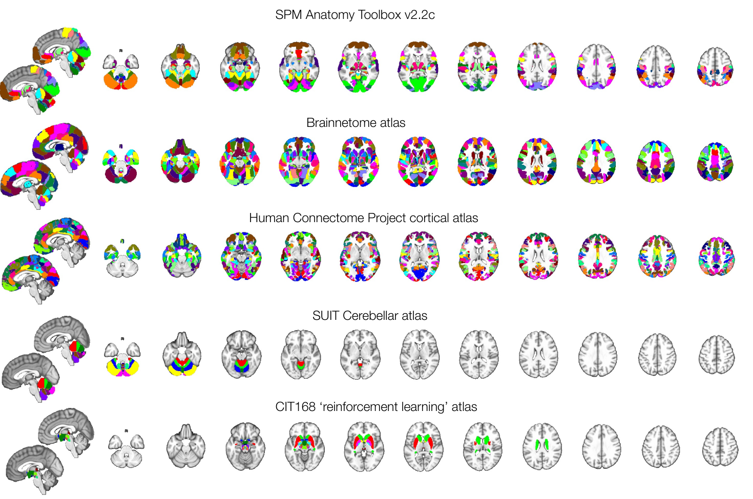
Examples of five different brain atlases, each constructed from specific brain properties. From top to bottom: the Jülich Brain / SPM Anatomy Toolbox (histology-based); the Brainnetome atlas (diffusion tractography-based); the Human Connectome Project multi-modal cortical atlas; the SUIT histology-based cerebellar atlas; and the CIT168 “reinforcement learning” atlas of selected subcortical regions. (Figure 23.1 from the book. © the authors and MIT Press; reproduced with permission — not covered by this site’s CC-BY license.)
Atlases are also the principled way to define regions of interest (ROIs). An ROI analysis averages the signal over the voxels in each parcel:
ȳⱼ — average signal in region j · Rⱼ — set of voxels in region j · |Rⱼ| — number of voxels in the region · yᵥ — data value at voxel v
where is the average signal in region , the set of voxels belonging to that region, the number of voxels it contains, and the data value at voxel .
Averaging boosts signal-to-noise and shrinks the multiple-comparisons problem from ~100,000 voxel tests to a handful of region tests. But how the ROI is chosen determines whether the analysis is valid. An a priori ROI — chosen from an atlas, an independent dataset, or an independent contrast before looking at the data being tested — yields unbiased estimates and honest P values. A post hoc ROI selected because it showed the strongest effect in the same data is circular (non-independent): selection by the maximum guarantees inflated effect sizes and can manufacture “significant” effects from pure noise. The hands-on lab makes this bias visible by simulation.
Even with a good atlas, localization has limits. The anatomical underlay may not match the functional data — the two are subject to different distortions, and distortions differ across studies — so rather than overlaying results on the single-subject Colin brain or the MNI-152, a better practice is to register your own participants’ T1 images to the reference space and build a group-average anatomical underlay from the study sample. This gives a closer match and reveals alignment precision: poor alignment shows up as blur or “ghosting” (multiple brain edges). Finally, activations cannot be definitively localized to small structures — the habenula, locus coeruleus, ventral tegmental area, and other small nuclei — at standard field strengths, because of physiological noise, differential distortion, and the intrinsic blurriness of BOLD. Localizing small structures is aided by high-field (7T+) imaging, structure-specific inter-subject registration (e.g., of the brainstem or cerebellum), and localization based on high-resolution functional rather than anatomical images. One need not refuse to interpret small nuclei at 1.5T or 3T, but strong claims should be avoided.
Hands-on tutorial
In this tutorial you will work with atlases and standard spaces from both ends: visualizing results in MNI template space, and extracting per-region averages for an ROI analysis. The full labs then demonstrate the circularity problem by simulation.
Step 1 — Load a standard template or atlas and visualize results in it. In Python we load the bundled MNI152 template and overlay a simulated statistic map placed at a known MNI coordinate; in MATLAB we load the CANlab combined 2018 atlas (Glasser cortex + Pauli basal ganglia + Morel thalamus + Diedrichsen cerebellum and more) and display its parcels.
% Requires CanlabCore + SPM12 on your MATLAB path
% Adapted from CANlab tutorials (github.com/canlab/CANlab_help_examples)

% Load the "CANlab combined 2018" atlas: ~500 labeled parcels in MNI space
atlas_obj = load_atlas('canlab2018_2mm');

% See all named atlases you can load (Glasser, Schaefer, Yeo, ...)
help load_atlas

orthviews(atlas_obj);        % interactive orthogonal slices
o2 = montage(atlas_obj);     % slice montage of all parcels
import numpy as np, nibabel as nib
from nilearn.datasets import load_mni152_template
from nilearn import plotting
from scipy.ndimage import gaussian_filter
template = load_mni152_template(resolution=2) # resolution = 2 mm voxels; bundled with nilearn, no download
plotting.plot_anat(template, title="MNI152 template")
# Simulated "activation" at right anterior insula, MNI (38, 22, -2)
ijk = np.linalg.inv(template.affine) @ [38, 22, -2, 1] # mm -> voxel
stat = np.zeros(template.shape)
stat[tuple(np.round(ijk[:3]).astype(int))] = 1.0
stat = gaussian_filter(stat, sigma=2.5) # sigma = 2.5 voxels (~5 mm): spread the focus like a smoothed blob
stat_img = nib.Nifti1Image(6 * stat / stat.max(), template.affine) # rescale so the peak "t" = 6
plotting.plot_stat_map(stat_img, bg_img=template, threshold=2.0, # threshold = 2.0: hide sub-threshold voxels
cut_coords=(38, 22, -2), title="Simulated result")Example output: (Python)
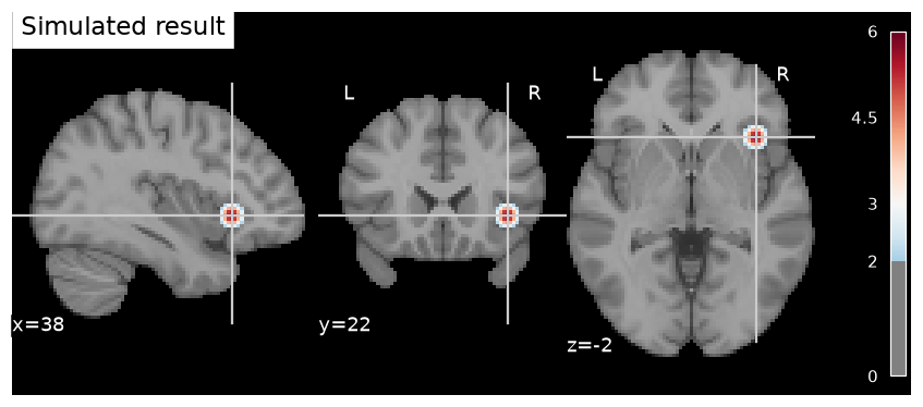
The simulated “activation” overlaid on the MNI152 template. The crosshairs sit at MNI — exactly the millimeter coordinate we specified, converted to voxel indices through the image affine.
Step 2 — Extract ROI averages and test them. ROI analysis averages the data over each region’s voxels, then runs one test per region. The key rule: choose the regions a priori — from an atlas or independent data — not because they “lit up” in the data you are about to test.
% Bundled sample data: 30 subjects, [reappraise - look] contrast images
image_obj = load_image_set('emotionreg');

% A priori selection: all thalamic parcels, chosen by name from the atlas
thal = select_atlas_subset(atlas_obj, {'Thal'});

% Average over each region's voxels, for every subject image
r = extract_roi_averages(image_obj, thal);
roi_avgs = cat(2, r.dat);                      % subjects x regions

% Plot each region with a one-sample t-test per column
barplot_columns(roi_avgs, 'names', format_strings_for_legend(thal.labels));
xlabel('Thalamic region'); ylabel('Contrast value');
from scipy import stats
rng = np.random.default_rng(0) # seed = 0 so the result is reproducible
# Parcel averages for 20 subjects x 6 parcels, with NO true effect anywhere
n_sub, n_parcels = 20, 6 # n_sub = subjects; n_parcels = a priori regions tested
roi_avgs = rng.standard_normal((n_sub, n_parcels))
t, p = stats.ttest_1samp(roi_avgs, 0) # one test per parcel
# A priori ROI (parcel 1, chosen before seeing the data): honest result
print(f"a priori ROI (parcel 1): t = {t[0]:+.2f}, p = {p[0]:.3f}")
# Circular ROI (the strongest parcel in this same data): biased!
best = int(np.argmax(t))
print(f"circular ROI (parcel {best + 1}): t = {t[best]:+.2f}, p = {p[best]:.3f}"
" <- selected BECAUSE it is the maximum")Example output: (Python)
a priori ROI  (parcel 1): t = -0.06, p = 0.955
circular ROI  (parcel 6): t = +3.02, p = 0.007  <- selected BECAUSE it is the maximum
In the Python data there is no signal at all, yet the “winning” parcel returns , — a publishable-looking effect conjured from noise, while the a priori parcel behaves honestly (, ). Selection and estimation must be independent.
The full labs go further: building a toy whole-brain parcellation in MNI space, comparing voxelwise and parcel-level group maps, quantifying circularity bias over thousands of null simulations (and fixing it with split-half selection), and — in MATLAB — auto-labeling a thresholded map with region.table() and rendering results on 3-D cortical surfaces.
Open the full Python lab notebook → or download the MATLAB live script, which mirrors it using CANlab atlas tools.


Thought questions
Two labs both report “dlPFC” activation, but their clusters do not overlap at all. Using the analogy between atlas regions and genes, explain what is lost when studies use informal labels — and what concretely changes for meta-analysis and theory-building when both labs instead report, say, Glasser area 8C with an atlas version number.
You are studying emotion processing in 7-year-olds but your pipeline warps every child’s brain to the adult MNI-152 template and applies adult atlas labels. Trace the specific errors this could introduce, and explain why even a perfect pediatric template would not fully resolve the ambiguity of claiming two groups activated “the same area.”
A colleague argues: “Circular ROI analysis isn’t a real problem — I corrected for multiple comparisons in my whole-brain map first, so the region is real; I’m just describing its effect size.” What is right and wrong in this argument? Which quantities remain biased after whole-brain correction, and what would you do instead?
Your 3T study shows a small cluster you believe is the locus coeruleus. What are three distinct reasons this localization could be wrong, and what combination of acquisition, registration, and reporting choices would let you make the claim more responsibly?
Histological, functional-connectivity, and multi-modal parcellations can carve the same cortex into quite different regions. For a study of individual differences in cerebellar contributions to working memory, which atlas family would you choose and why — and how would your inference change if your effect straddles a parcel boundary in one atlas but not another?
Quiz yourself
Q1. What is a brain atlas, and what two things does it provide that make findings comparable across studies?
Answer: An atlas is a standard brain labeled with regions and their boundaries, defined from properties such as histology, connectivity, or prior findings. It provides uniform neuroanatomical labels and precisely defined units of analysis, so activations from different studies can be assigned to the same named region and integrated directly.
Q2. What is the difference between a fixed-label atlas and a probabilistic atlas?
Answer: A fixed-label atlas assigns each voxel to a single structure (it is either in the putamen or not). A probabilistic atlas gives, for each voxel, the likelihood that it belongs to each structure, estimated from a set of individually labeled brains — capturing anatomical variability across people.
Q3. How was MNI space created, and how does it relate to the Talairach atlas?
Answer: The MNI averaged T1 images from 305 young healthy adults, each mapped onto the Talairach template, producing the MNI-305 composite — the original definition of MNI space with stereotaxic (x, y, z) coordinates. Later refinements include the Colin-27 (one subject scanned 27 times), the MNI-152 (better contrast and coverage), and the ICBM-452.
Q4. Why can surface-based templates like fsaverage or fs_LR align cortex more accurately than volumetric registration?
Answer: Surface templates inflate or flatten the cortical sheet and align brains using landmarks and continuous contours along the surface itself. Because cortical folding varies greatly between people, matching the 2-D sheet respects cortical topology in a way that warping 3-D volumes cannot, so when a clean cortical surface is available, surface alignment is appreciably more accurate in cortex.
Q5. Name the major families of brain atlases and one example of each.
Answer: Histology-based (Brodmann areas; the Jülich Brain / SPM Anatomy Toolbox); structural template-based (MNI-152, ICBM-452); functional connectivity-based (Yeo–Buckner and Schaefer parcellations); diffusion-based (ICBM-DTI-81 white-matter atlas, Brainnetome); meta-analysis-based (Neurosynth, Neuroquery); and multi-modal (the Glasser HCP atlas, 180 areas per hemisphere from folding, myelin, connectivity, and task maps).
Q6. What makes an ROI analysis “circular,” and what is the consequence?
Answer: Circularity (non-independence) arises when the ROI is selected using the same data that are then used to estimate or test the effect — for example, picking the parcel with the largest t statistic and reporting its effect size. Selection by the maximum guarantees upwardly biased effect estimates and invalid P values, and can produce apparently large “effects” from pure noise. Valid alternatives: a priori atlas ROIs, independent datasets or contrasts, or split-half/cross-validated selection.
Q7. Why is it better to build a group-average anatomical underlay from your own study sample than to display results on the Colin brain or MNI-152?
Answer: The study’s functional images have their own distortion pattern, which differs from any standard template. A group-average T1 from the same participants matches the functional data more closely, and it doubles as a diagnostic: if inter-subject alignment is poor, the average appears blurry or shows “ghosting” — multiple brain boundaries from misaligned images.
Q8. Why can’t fMRI activations be definitively localized to small nuclei like the habenula or locus coeruleus in standard 3T studies, and what three approaches help?
Answer: Physiological noise artifacts, differential distortion between functional and anatomical images, and the intrinsic blurriness of BOLD all exceed the size of such structures. Localization is aided by (a) high-field imaging (7T or above), (b) inter-subject registration targeted to specific structures such as the brainstem or cerebellum, and (c) localizing on high-resolution functional images rather than anatomical ones. Interpret small nuclei cautiously and avoid strong claims at standard field strength.
 The book: Elements of Functional Magnetic Resonance Imaging — Wager & Lindquist, MIT Press