Chapter 23 Lab — Localizing and Interpreting Results (Python) - Elements of fMRI Analysis

Group analyses give you a statistic map; interpretation begins when you place that map in a standard coordinate space and relate it to brain atlases and parcellations. In this lab you will:

Explore MNI space: load the MNI152 template and convert between millimeter coordinates and voxel indices with the image affine
Simulate a group activation map at known MNI coordinates and overlay it on the template
Build a toy parcellation of the template — a stand-in for a real atlas
Run an ROI analysis: extract per-subject parcel averages and test them, comparing parcel-level with voxelwise inference
Quantify circularity bias: show by simulation that post hoc (circular) ROI selection inflates effects even in pure noise — and that split-half selection fixes it

Everything is simulated in template space, so no datasets are downloaded and every step has a known ground truth.

How to run this notebook. Run it in your browser from the tutorial site, in Google Colab, or in a local Jupyter environment with numpy, scipy, matplotlib, scikit-learn, statsmodels, nibabel, and nilearn installed. See the chapter page for the concepts behind each step.

▶ This notebook is interactive. Click the ⏻ power icon at the top right of this page to run it in your browser — no installation needed (the kernel takes ~30–60 s to start the first time). Then run cells top to bottom, starting with the first code cell below: later cells depend on the imports and variables defined earlier, and will error if you skip ahead.

# Setup — installs nilearn when it's missing (safe to re-run anywhere)
try:
    import nilearn  # noqa: F401 — already present on many local setups
except ImportError:
    import sys
    if "pyodide" in sys.modules:
        # Running in your browser (JupyterLite): install a browser-compatible version
        import piplite
        await piplite.install("nilearn==0.13.1")
    else:
        # Colab or local Python
        import subprocess
        subprocess.check_call([sys.executable, "-m", "pip", "install", "-q", "nilearn"])
print("nilearn ready:", __import__("nilearn").__version__)

nilearn ready: 0.14.0

import numpy as np
import matplotlib.pyplot as plt
import nibabel as nib
from scipy import stats
from scipy.ndimage import gaussian_filter

from nilearn.datasets import load_mni152_template
from nilearn import plotting
from sklearn.cluster import MiniBatchKMeans
from statsmodels.stats.multitest import multipletests

rng = np.random.default_rng(23)
np.set_printoptions(precision=3, suppress=True)
print("numpy", np.__version__)

numpy 2.4.6

Part 1 — MNI space: templates, affines, and coordinates¶

Reporting a result at MNI $(x, y, z) = (38, 22, -2)$ only means something because everyone’s data have been warped to a shared template. The MNI152 template — an average of 152 co-registered T1 scans from young healthy adults — is bundled with nilearn, so we can load it without downloading anything.

Every NIfTI image carries an affine matrix that maps voxel indices $(i, j, k)$ to millimeter coordinates $(x, y, z)$ in the template’s stereotaxic space. This little piece of bookkeeping is what makes coordinate reporting, atlas lookup, and cross-study comparison possible.

template = load_mni152_template(resolution=2)   # resolution = 2 mm voxels; bundled with nilearn, no download

print("Image shape (voxels):", template.shape)
print("Voxel size (mm):     ", template.header.get_zooms())
print("Affine (voxel -> mm):\n", template.affine)

plotting.plot_anat(template, cut_coords=(0, 0, 0),
                   title="MNI152 template (origin = anterior commissure)")
plt.show()

Image shape (voxels): (99, 117, 95)
Voxel size (mm):      (np.float32(2.0), np.float32(2.0), np.float32(2.0))
Affine (voxel -> mm):
 [[   2.    0.    0.  -98.]
 [   0.    2.    0. -134.]
 [   0.    0.    2.  -72.]
 [   0.    0.    0.    1.]]

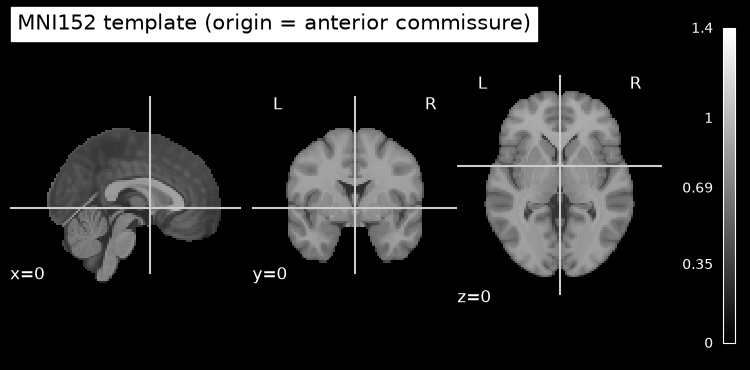
The affine’s diagonal gives the voxel size (2 mm here); the last column gives the mm coordinate of voxel $(0,0,0)$ . Multiplying by the affine converts voxel indices to mm; multiplying by its inverse goes the other way. We will need both directions constantly — atlases and results are stored on voxel grids, but coordinates are reported in mm.

affine = template.affine
inv_affine = np.linalg.inv(affine)

def mm_to_voxel(xyz_mm):
    '''Convert an MNI (x, y, z) coordinate in mm to voxel indices (i, j, k).'''
    ijk = inv_affine @ np.append(xyz_mm, 1.0)
    return np.round(ijk[:3]).astype(int)

def voxel_to_mm(ijk):
    '''Convert voxel indices (i, j, k) to MNI mm coordinates.'''
    return (affine @ np.append(ijk, 1.0))[:3]

r_insula = np.array([38, 22, -2])          # right anterior insula (MNI, mm)
ijk = mm_to_voxel(r_insula)
print("MNI", r_insula, "mm  ->  voxel indices", ijk)
print("Round trip:", voxel_to_mm(ijk), "mm")

MNI [38 22 -2] mm  ->  voxel indices [68 78 35]
Round trip: [38. 22. -2.] mm

Part 2 — A simulated group effect at known MNI coordinates¶

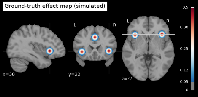
We now create a ground-truth effect map: three activation foci placed at MNI coordinates typical of a pain/salience contrast — dorsal anterior cingulate and bilateral anterior insula. Because we build it ourselves, we will later be able to check exactly which parcels should show effects.

The peak effect is 0.5 in units of the between-subject noise SD (a moderate effect size, $d = 0.5$ at the peak).

tdata = template.get_fdata()
brain_mask = tdata > 0.2 * tdata.max()          # keep voxels above 20% of max intensity: crude brain mask
print(f"{brain_mask.sum():,} voxels in the brain mask")

foci_mm = {"dACC":         (0, 20, 36),
           "R ant insula": (38, 22, -2),
           "L ant insula": (-36, 20, -4)}

truth = np.zeros(template.shape)
for name, xyz in foci_mm.items():
    truth[tuple(mm_to_voxel(xyz))] = 1.0
truth = gaussian_filter(truth, sigma=2.5)       # sigma = 2.5 voxels: spread each focus over ~10 mm
truth = 0.5 * truth / truth.max()               # peak effect = 0.5 (noise SD = 1)
truth *= brain_mask

truth_img = nib.Nifti1Image(truth, affine)
plotting.plot_stat_map(truth_img, bg_img=template, threshold=0.05,
                       cut_coords=foci_mm["R ant insula"],
                       title="Ground-truth effect map (simulated)")
plt.show()

235,398 voxels in the brain mask

Part 3 — Build a toy parcellation¶

A parcellation divides the brain into non-overlapping labeled regions. Real atlases derive their boundaries from histology (Jülich), functional connectivity (Yeo–Buckner, Schaefer), diffusion tractography (Brainnetome), meta-analysis (Neurosynth), or multiple modalities combined (the Glasser HCP atlas).

Here we build a deliberately naive one — 60 spatially compact parcels from k-means clustering of voxel coordinates only. It knows nothing about anatomy or function, but it plays the same computational role as a real atlas: an integer label image on the template grid, defined independently of the data we will analyze. That independence is what makes it legitimate for a priori ROI selection.

ijk_brain = np.array(np.where(brain_mask)).T                 # in-brain voxel indices
xyz_brain = ijk_brain @ affine[:3, :3].T + affine[:3, 3]     # ... in mm

n_parcels = 60                                               # number of parcels in the toy atlas
km = MiniBatchKMeans(n_clusters=n_parcels, random_state=0,   # random_state = 0: reproducible clustering
                     n_init=3, batch_size=2048)              # 3 restarts; 2048 voxels per mini-batch
parcel_of_voxel = km.fit_predict(xyz_brain)                  # 0 .. n_parcels-1

label_data = np.zeros(template.shape, dtype=np.int32)
label_data[brain_mask] = parcel_of_voxel + 1                 # 0 = background
label_img = nib.Nifti1Image(label_data, affine)

plotting.plot_roi(label_img, bg_img=template,
                  title=f"Toy parcellation ({n_parcels} spatial parcels)")
plt.show()

# Which parcels contain our true foci? (ground truth for later)
true_parcels = {name: int(label_data[tuple(mm_to_voxel(xyz))])
                for name, xyz in foci_mm.items()}
print("Parcels containing the true foci:", true_parcels)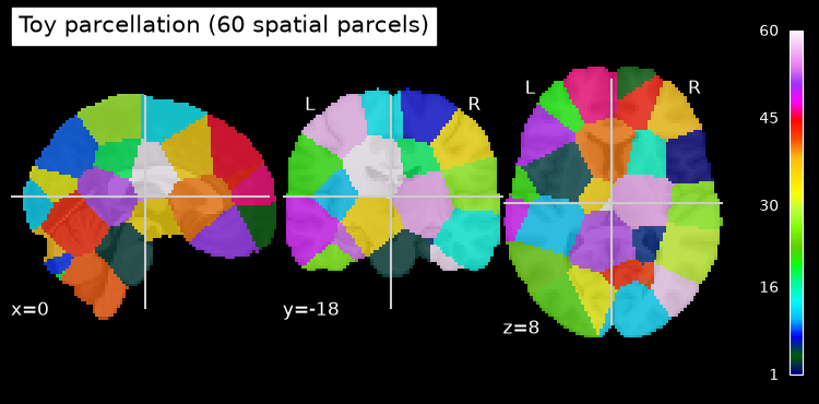

Parcels containing the true foci: {'dACC': 36, 'R ant insula': 24, 'L ant insula': 55}

Part 4 — ROI analysis: parcel averages vs. voxelwise tests¶

We simulate a group study: 20 subjects, each with a contrast map equal to the true effect (scaled by a subject-specific amplitude) plus independent noise. Then we analyze it two ways:

Voxelwise: a one-sample t-test at every in-brain voxel (~230,000 tests)
ROI analysis: average each subject’s map within each parcel, then one t-test per parcel (60 tests)

The parcel average for subject $s$ in region $j$ is

\bar{y}_{sj} = \frac{1}{|R_j|}\sum_{v \in R_j} y_{sv}

(1)

ȳₛⱼ — parcel average for subject s, region j · Rⱼ — set of voxels in parcel j · |Rⱼ| — number of voxels in the parcel · yₛᵥ — subject s’s contrast value at voxel v

where $\bar{y}_{sj}$ is subject $s$ ’s average over region $j$ , $R_j$ the set of voxels in parcel $j$ , $|R_j|$ the number of voxels it contains, and $y_{sv}$ the subject’s contrast value at voxel $v$ .

Averaging over a parcel’s voxels suppresses voxel-level noise, and testing 60 parcels instead of 230,000 voxels makes multiple-comparisons correction far less punishing.

n_sub = 20                                          # number of simulated subjects
truth_vec = truth[brain_mask]                       # true effect per in-brain voxel
amp = 1 + 0.3 * rng.standard_normal(n_sub)          # subject amplitudes ~ N(1, 0.3)
noise = rng.standard_normal((n_sub, truth_vec.size))
subject_maps = amp[:, None] * truth_vec[None, :] + noise    # subjects x voxels

# --- Voxelwise group t map ---
t_vox = subject_maps.mean(0) / (subject_maps.std(0, ddof=1) / np.sqrt(n_sub))

t_vox_data = np.zeros(template.shape)
t_vox_data[brain_mask] = t_vox
plotting.plot_stat_map(nib.Nifti1Image(t_vox_data, affine), bg_img=template,
                       threshold=3.5, cut_coords=foci_mm["R ant insula"],
                       title="Voxelwise group t map (thresholded |t| > 3.5)")
plt.show()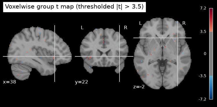

# --- Parcel-level ROI analysis ---
counts = np.bincount(parcel_of_voxel, minlength=n_parcels)
roi_means = np.vstack([
    np.bincount(parcel_of_voxel, weights=subject_maps[s], minlength=n_parcels) / counts
    for s in range(n_sub)
])                                                   # subjects x parcels

t_roi, p_roi = stats.ttest_1samp(roi_means, 0)
sig_fdr = multipletests(p_roi, alpha=0.05, method="fdr_bh")[0]

order = np.argsort(t_roi)[::-1]
print("Top parcels by t (FDR-significant marked *):")
for j in order[:8]:
    mark = "*" if sig_fdr[j] else " "
    print(f"  parcel {j + 1:3d}{mark}  t = {t_roi[j]:5.2f}   p = {p_roi[j]:.2g}")
print("\nParcels that truly contain foci:", sorted(set(true_parcels.values())))

# Paint the parcel t values back onto the brain for display
t_parcel_data = np.zeros(template.shape)
t_parcel_data[brain_mask] = t_roi[parcel_of_voxel]
plotting.plot_stat_map(nib.Nifti1Image(t_parcel_data, affine), bg_img=template,
                       threshold=3.0, cut_coords=foci_mm["R ant insula"],
                       title="Parcel-level t map (each parcel = one test)")
plt.show()

Top parcels by t (FDR-significant marked *):
  parcel  36*  t =  8.64   p = 5.2e-08
  parcel  55*  t =  6.78   p = 1.8e-06
  parcel  24*  t =  4.78   p = 0.00013
  parcel  19   t =  2.14   p = 0.045
  parcel  45   t =  2.01   p = 0.059
  parcel  31   t =  1.98   p = 0.063
  parcel  35   t =  1.89   p = 0.074
  parcel  57   t =  1.77   p = 0.092

Parcels that truly contain foci: [24, 36, 55]

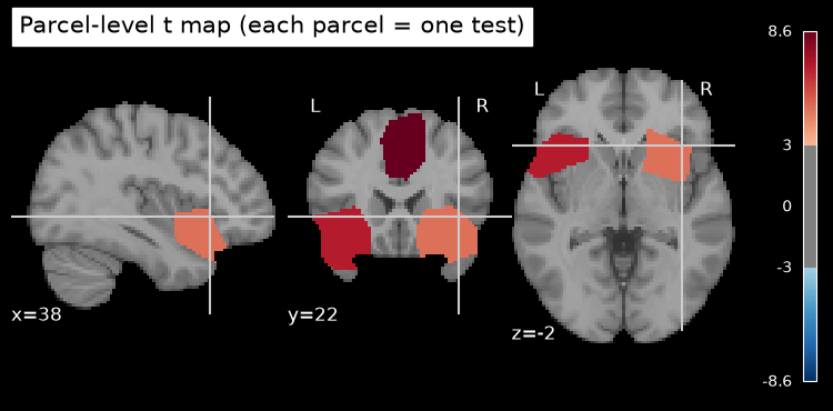
The FDR-significant parcels should be exactly (or nearly) the ones containing the simulated foci. Two things to notice:

The parcel-level map is blocky — each parcel gets one value. That is the tradeoff: fewer, more powerful tests, at the cost of spatial resolution and the risk that an effect straddles a parcel boundary or occupies only a small fraction of a large parcel (diluting its average).
In real analyses the parcels would come from a published atlas registered to the same MNI space, and you would report which atlas and which version you used — that is what makes ROI results comparable across studies.

Part 5 — The circularity trap: a priori vs. post hoc ROI selection¶

Now the cautionary tale. Suppose a researcher runs a study with no true effect anywhere, looks at the parcel-level results, picks the parcel with the largest t statistic, and reports its effect size “because that’s where the effect was.”

That analysis is circular (non-independent): the same noise that makes a parcel the maximum also inflates its estimated effect. We quantify the bias over 2,000 simulated null studies, comparing:

A priori ROI: parcel 1, chosen before seeing any data → unbiased
Circular ROI: the parcel with the maximum t in the same data → biased

n_sims, n_sub_c, n_parc_c = 2000, 20, 60   # n_sims = null studies; n_sub_c = subjects; n_parc_c = parcels

null_data = rng.standard_normal((n_sims, n_sub_c, n_parc_c))   # truth = 0 everywhere
m  = null_data.mean(axis=1)
se = null_data.std(axis=1, ddof=1) / np.sqrt(n_sub_c)
t  = m / se

apriori_est  = m[:, 0]                                  # parcel chosen in advance
best         = np.argmax(t, axis=1)                     # parcel chosen post hoc
circular_est = m[np.arange(n_sims), best]
circular_t   = t[np.arange(n_sims), best]

t_crit = stats.t.ppf(0.975, df=n_sub_c - 1)
fp_apriori  = np.mean(np.abs(t[:, 0]) > t_crit)
fp_circular = np.mean(np.abs(circular_t) > t_crit)

print(f"Mean estimated effect (truth = 0):  a priori {apriori_est.mean():+.3f}   "
      f"circular {circular_est.mean():+.3f}")
print(f"'Significant' at p < .05 (truth = 0):  a priori {fp_apriori:.1%}   "
      f"circular {fp_circular:.1%}")

fig, ax = plt.subplots(figsize=(7, 4))
bins = np.linspace(-0.6, 1.0, 50)
ax.hist(apriori_est, bins, alpha=0.6, label="A priori ROI (parcel 1)")
ax.hist(circular_est, bins, alpha=0.6, label="Circular ROI (max of same data)")
ax.axvline(0, color="k", lw=1)
ax.set_xlabel("Estimated effect (true effect = 0)")
ax.set_ylabel("Number of simulated studies")
ax.set_title("Circular ROI selection inflates effects in pure noise")
ax.legend()
plt.tight_layout()
plt.show()

Mean estimated effect (truth = 0):  a priori +0.007   circular +0.489
'Significant' at p < .05 (truth = 0):  a priori 5.3%   circular 77.2%

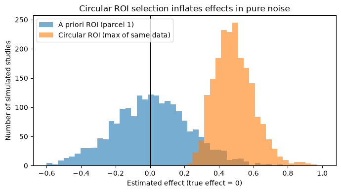
With no true effect anywhere, the circular estimate averages around +0.4 noise-SD units and is “significant” essentially every time — a textbook machine for manufacturing findings. The a priori ROI behaves exactly as statistics promises: centered on zero, with a ~5% false positive rate.

The fix is independence between selection and estimation. Besides using atlas ROIs defined in advance, a simple in-study remedy is split-half selection: choose the ROI with one half of the subjects, estimate the effect in the other half.

half1, half2 = null_data[:, :10], null_data[:, 10:]   # split the 20 subjects into two halves of 10

t_half1 = half1.mean(1) / (half1.std(1, ddof=1) / np.sqrt(10))
sel = np.argmax(t_half1, axis=1)                    # select on half 1 ...
holdout_est = half2.mean(1)[np.arange(n_sims), sel] # ... estimate on half 2

print(f"Mean estimated effect in held-out half (truth = 0): {holdout_est.mean():+.3f}")
print(f"Compare: circular estimate in the same data:        {circular_est.mean():+.3f}")

Mean estimated effect in held-out half (truth = 0): +0.006
Compare: circular estimate in the same data:        +0.489

Summary¶

The affine links voxel grids to standard-space mm coordinates; MNI space is a shared frame built from group-average templates (MNI-305 → MNI-152 → ICBM-452).
Parcellations turn the brain into named units of analysis. Real atlases encode histology, connectivity, meta-analysis, or multi-modal information — our toy k-means version shows the mechanics.
ROI analysis (parcel averaging + one test per region) trades spatial resolution for power and a lighter multiple-comparisons burden.
ROI selection must be independent of the data being tested: use a priori atlas ROIs, independent contrasts or datasets, or split-half/cross-validated selection. Circular selection inflates effects even in pure noise.

Explore further. Nilearn’s nilearn.datasets module can fetch real atlases (Schaefer, Harvard–Oxford, Yeo, Destrieux) and nilearn.maskers.NiftiLabelsMasker automates parcel extraction on real data. Neurosynth (neurosynth.org), Neuroquery (neuroquery.org), and neuromaps offer meta-analytic and multi-modal annotation; the CANlab tools (canlab.github.io) mirror this workflow in MATLAB with atlas objects and automatic labeling via region.table().