Contrasts and Inference with the GLM
Run this code: ⚡ In-browser lab · Colab · MATLAB Online
Overview
Once the GLM parameters have been estimated (Chapter 18), the scientific work begins: testing whether the response to a single task differs from zero, whether two conditions differ in activation magnitude, whether a set of nuisance covariates explains significant variance, or whether the main effects and interaction of a factorial design are present. All of these questions are answered with statistical tests of contrasts — linear combinations of the values.
Consider a task with two conditions, A and B — say, viewing famous versus non-famous faces — each modeled by one regressor, with the intercept as another column. The comparison “A − B” corresponds to a contrast vector with a +1 for A, a -1 for B, and 0 for the intercept. The contrast estimate is obtained by applying the weights to the parameter estimates:
ĉ — estimated contrast value · c — vector of contrast weights (one per model parameter) · β̂ — estimated GLM coefficients
where is the estimated contrast value, the vector of contrast weights (one weight per model parameter), and the vector of estimated GLM coefficients from Chapter 18.
and testing against . Contrasts can encode any pre-specified question: the response to a single condition ( over the task betas), the average of several conditions (), or any difference among them.
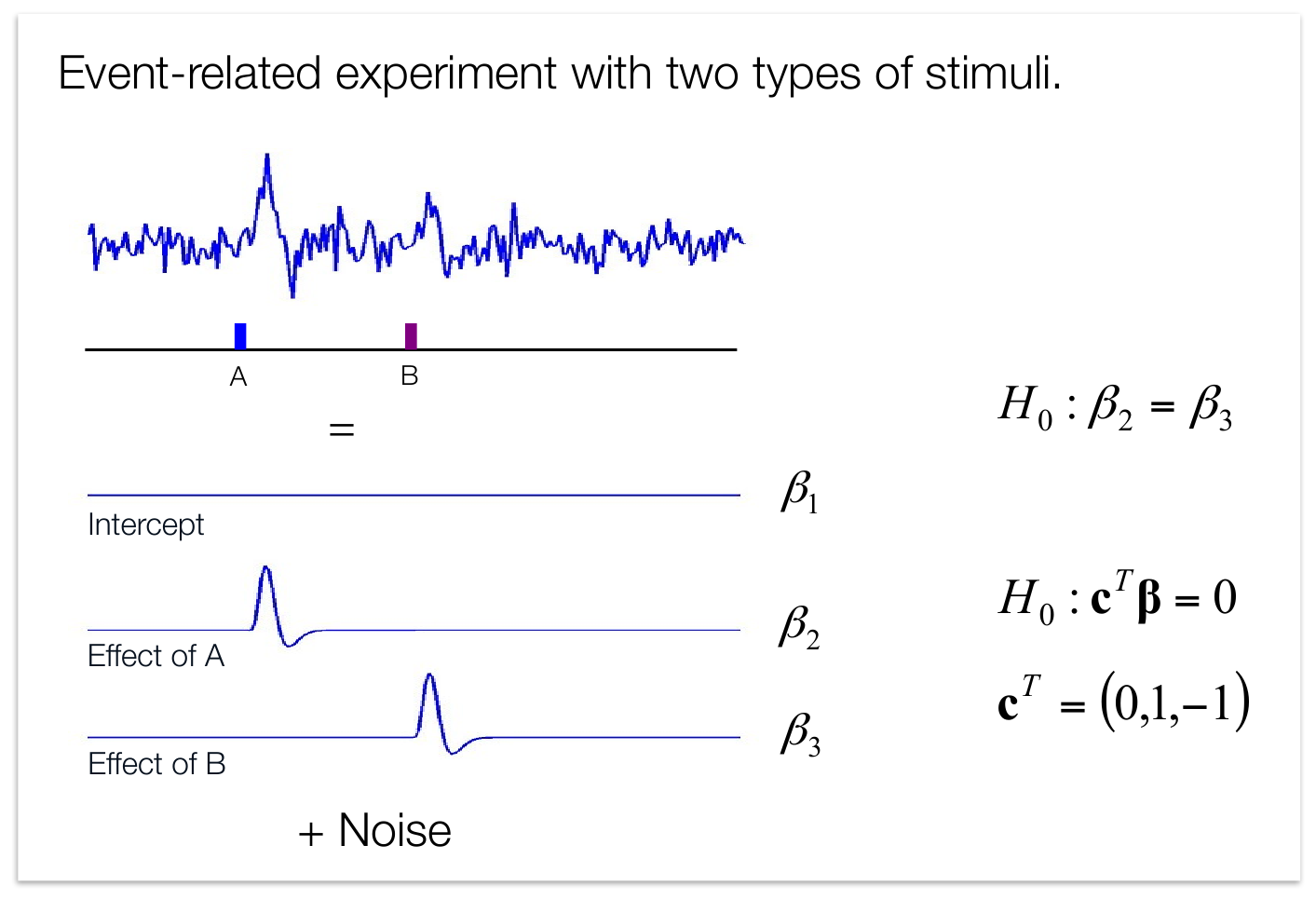
A simple t-contrast. Conditions A and B have regression coefficients and (the intercept is ). The contrast estimates the activation difference between conditions, testing — equivalently . (Figure 20.1 from the book. © the authors and MIT Press; reproduced with permission — not covered by this site’s CC-BY license.)
A few rules of thumb govern contrast weights. Differences between conditions should use weights that sum to zero (), so that the expected contrast value is 0 under the null hypothesis of equal responses. Tests against the implicit baseline need not sum to zero (e.g., or ): each is already 0 under the null, so any average of them is too. Scaling the weights changes the magnitude of the contrast estimate but not the inference — appears in both the numerator and denominator of the t-statistic, so and yield identical t- and P-values. Two exceptions make scale worth caring about anyway: if you report activation in meaningful units (e.g., percent signal change), scale the weights so the positive weights sum to +1 and the negative weights to -1, making the contrast a difference of condition means; and the scale of must be identical across all participants entering a group analysis — if some participants are missing runs, their weights must be re-normalized, or scale differences will masquerade as noise at the second level. A related caveat is estimability: not every linear function of the parameters has a linear unbiased estimator. In a one-way ANOVA parameterized as — where is the grand mean, the effect of condition , and the error for observation in condition — neither nor an individual is uniquely estimable, but and are — the model can only answer questions about combinations the design distinguishes.
Contrasts also bring analysis of variance into the GLM framework. In a factorial repeated-measures design — very common in fMRI — each cell of the design is modeled as its own condition, and contrasts recover the classical effects. With four cells A–D from crossing [famous vs. non-famous] × [upright vs. inverted], the contrast tests the main effect of fame, the main effect of orientation, and their interaction.
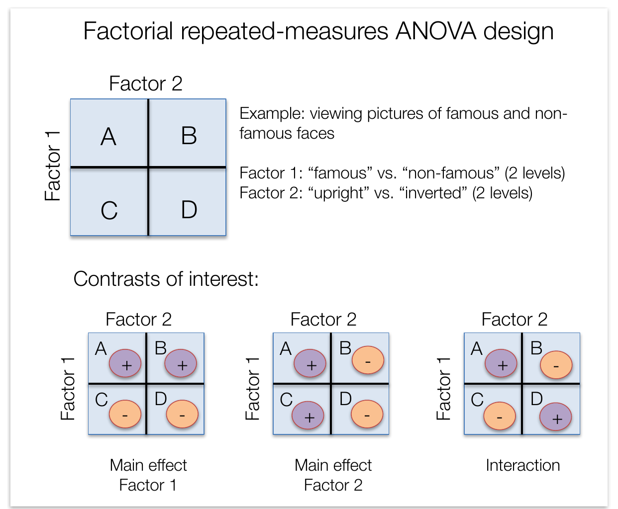
A factorial repeated-measures ANOVA design. (Top) Two factors with two levels each — [famous vs. non-famous] × [upright vs. inverted] — yield four cells, A–D, each modeled as its own event type. (Bottom) Contrast weight patterns for the main effect of each factor and their interaction: purple plus signs are +1, orange minus signs are -1. (Figure 20.2 from the book. © the authors and MIT Press; reproduced with permission — not covered by this site’s CC-BY license.)
Contrasts with a single column — one model degree of freedom — are t-contrasts. Analysis packages write the resulting contrast values at every voxel to disk as contrast images (also called COPEs, contrasts of parameter estimates), which become the inputs to group analysis (Chapter 21). An F-contrast instead specifies a contrast matrix whose columns define a subspace of effects to be tested jointly. F-tests are non-directional and unsigned — positive and negative deviations both increase significance — and they shine in three situations: (1) testing whether a block of correlated nuisance covariates (e.g., six head-motion parameters) together explains significant variance, even when no single one does; (2) omnibus tests of a whole model or ANOVA (both main effects and the interaction at once); and (3) testing condition differences when the HRF is modeled with multiple basis functions. The last case matters because betas for different basis functions are incommensurate — “apples and oranges,” mixing amplitude and shape information — so they cannot simply be averaged; the F-test assesses their joint difference instead, and significant regions require post hoc inspection to see how conditions differ.
Inference for a t-contrast uses the same machinery as for a single beta. Under the null, has mean 0 and variance (with the appropriate GLS analogue when errors are prewhitened; Chapter 19), giving
t — t-statistic for the contrast · c — contrast weights · β̂ — estimated coefficients · σ̂² — estimated error variance · X — design matrix (time × predictors)
where is the contrast estimate, the estimated error variance, the design matrix, and the denominator as a whole the standard error of the contrast.
which follows an approximate t-distribution under with (error) degrees of freedom. For an F-contrast, the full model is compared with a reduced model whose design matrix omits the subspace spanned by the contrasts — the F-statistic asks how much extra variance the effects of interest explain:
F — F-statistic for the contrast · r₀ — reduced-model residuals · r — full-model residuals · ν₁ — number of independent effects tested · ν₂ — error degrees of freedom
where and are the reduced- and full-model residuals, the number of independent effects tested (the model degrees of freedom of the contrast), and the error degrees of freedom.
In the massively univariate approach, these statistics are computed at every voxel, producing the t- and F-maps that thresholding and multiple-comparisons procedures (Chapter 22) then operate on.
One final logical distinction rounds out the toolkit. An F-test asks whether any of a set of effects is nonzero — a logical OR. Many claims are logical AND claims: “this region responds to both famous and non-famous faces more than houses.” Such conjunction claims are validly tested with the minimum-statistic rule — every component contrast must individually exceed the significance threshold — not by a significant F, and not by one significant test plus one non-significant test. The labs below make this distinction concrete.
Hands-on tutorial
In this tutorial you will fit a three-condition GLM (A = famous faces, B = non-famous faces, C = houses) to a simulated voxel and ask it questions with contrasts. Because the simulation has known true betas (, , , intercept 100), every contrast has a known true value. Task regressors are scaled to peak at 1, so a beta of 1.0 is about a 1% signal change.
Step 1 — Fit a three-condition GLM. Build the design matrix by convolving each condition’s onsets with the canonical HRF (as in Chapter 18), simulate the voxel, and fit by OLS — saving the pieces every contrast test reuses: , , and .
% Requires CanlabCore + SPM12 on your MATLAB path
% Adapted from CANlab tutorials (github.com/canlab)
TR = 2; n_scans = 200;                        % 200 volumes, 400-s run
rng(2024);                                    % reproducible design and noise
all_onsets = (10:9:384)';                     % 42 events, 9 s apart
shuffled = all_onsets(randperm(42));          % randomly interleave A, B, C
ons = {sort(shuffled(1:14)), sort(shuffled(15:28)), sort(shuffled(29:42))};

X = onsets2fmridesign(ons, TR, n_scans * TR); % A, B, C, intercept (last)

% onsets2fmridesign scales the HRF to peak 1, so betas are ~% signal change
beta_true = [1.0 0.6 0.3 100]';               % A, B, C, intercept
y = X * beta_true + 0.15 * randn(n_scans, 1); % noise SD = 0.15% of baseline

beta_hat = (X' * X) \ (X' * y);               % OLS estimates
r       = y - X * beta_hat;
dfe     = n_scans - size(X, 2);               % error degrees of freedom
sigma2  = (r' * r) / dfe;                     % error variance estimate
XtX_inv = inv(X' * X);
disp(table(beta_true, beta_hat))
import numpy as np, pandas as pd
from scipy import stats
from nilearn.glm.first_level import make_first_level_design_matrix
t_r, n_scans = 2.0, 200 # 200 volumes, 400-s run
frame_times = np.arange(n_scans) * t_r # volume acquisition times (s)
rng = np.random.default_rng(2024) # reproducible design and noise
onsets = np.arange(10, 385, 9.0) # 42 events, 9 s apart
labels = rng.permutation(["A"] * 14 + ["B"] * 14 + ["C"] * 14)
events = pd.DataFrame({"onset": onsets, "duration": 1.0, "trial_type": labels})
X = make_first_level_design_matrix(frame_times, events,
hrf_model="spm", drift_model=None)
Xm = X.to_numpy(copy=True) # columns: A, B, C, constant
Xm[:, :3] /= Xm[:, :3].max(axis=0) # peak-normalize task columns
beta_true = np.array([1.0, 0.6, 0.3, 100.0]) # A, B, C, intercept
y = Xm @ beta_true + 0.15 * rng.standard_normal(n_scans) # noise SD = 0.15%
beta_hat = np.linalg.solve(Xm.T @ Xm, Xm.T @ y) # OLS estimates
resid = y - Xm @ beta_hat
dfe = n_scans - Xm.shape[1] # error degrees of freedom
sigma2 = resid @ resid / dfe # error variance estimate
XtX_inv = np.linalg.inv(Xm.T @ Xm)
print(pd.DataFrame({"true": beta_true, "estimate": beta_hat}, index=X.columns))Example output: (Python; MATLAB values differ slightly because the random streams differ)
           true   estimate
A           1.0   1.033275
B           0.6   0.588489
C           0.3   0.321265
constant  100.0  99.986921
Step 2 — Ask questions with t- and F-contrasts. Each t-contrast turns one question into one number: a pairwise difference (), a difference of means (faces − houses, ), and a task average versus baseline (). The F-contrast stacks and — two rows that span all pairwise differences — to ask whether the conditions differ from each other at all.
C = [1 -1 0 0; 0.5 0.5 -1 0; 1/3 1/3 1/3 0]';   % one contrast per COLUMN
con_val = C' * beta_hat;                          % contrast estimates
se_con  = sqrt(sigma2 * diag(C' * XtX_inv * C));  % contrast SEs
t_con   = con_val ./ se_con;                      % t-statistics
p_con   = 2 * (1 - tcdf(abs(t_con), dfe));        % two-tailed p-values
disp(table(con_val, t_con, p_con, 'RowNames', ...
    {'A - B', 'faces - houses', 'task avg vs baseline'}))

% F-contrast: do the conditions differ from each other at all?
L  = [1 -1 0 0; 0 1 -1 0];                        % one contrast per ROW
Lb = L * beta_hat;
F  = Lb' * ((L * XtX_inv * L') \ Lb) / (size(L, 1) * sigma2);
fprintf('any-difference F(2,%d) = %.2f, p = %.3g\n', ...
    dfe, F, 1 - fcdf(F, 2, dfe));
def t_contrast(c):
c = np.asarray(c, float)
value = c @ beta_hat
se = np.sqrt(sigma2 * c @ XtX_inv @ c)
return value, value / se
for name, c in [("A - B ", [1, -1, 0, 0]),
("faces - houses ", [0.5, 0.5, -1, 0]),
("task avg vs baseline", [1/3, 1/3, 1/3, 0])]:
value, t = t_contrast(c)
p = 2 * stats.t.sf(abs(t), dfe)
print(f"{name}: value = {value:+.3f}, t({dfe}) = {t:6.2f}, p = {p:.3g}")
# F-contrast: do the conditions differ from each other at all?
L = np.array([[1., -1, 0, 0], [0, 1, -1, 0]]) # one contrast per row
Lb = L @ beta_hat
F = Lb @ np.linalg.solve(L @ XtX_inv @ L.T, Lb) / (len(L) * sigma2)
print(f"any-difference F({len(L)},{dfe}) = {F:.2f}, "
f"p = {stats.f.sf(F, len(L), dfe):.3g}")Example output:
A - B               : value = +0.445, t(196) =  11.60, p = 5.11e-24
faces - houses      : value = +0.490, t(196) =  14.45, p = 1.03e-32
task avg vs baseline: value = +0.648, t(196) =  18.13, p = 8.63e-44
any-difference F(2,196) = 176.10, p = 1.68e-44
The pairwise and mean-difference contrasts recover their true values closely (about 0.45 and 0.49, against true values of 0.4 and 0.5), each with a large t, and the any-difference F is decisive — while ignoring the much larger activation that all three conditions share relative to baseline. The full labs continue the arc: contrast scaling and covariate centering, the equivalence of the contrast-matrix F and the full-versus-reduced-model F, for one-row contrasts, and a conjunction demo showing why “A and B” claims need the minimum-statistic rule.
Open the full Python lab notebook → or download the MATLAB live script, which mirrors it using CANlab tools.


Thought questions
A colleague reports that region X “activates to condition A” based on the contrast , and another lab, modeling the same data with a different set of unmodeled baseline periods, fails to replicate it — yet both labs agree perfectly on the contrast . Explain why, using the concepts of the implicit baseline and estimability, and state which kinds of claims are robust to baseline choices.
In a multi-run study, one participant’s scanner crashed after two of four runs, and the analyst simply zeroed out that participant’s missing-run contrast weights without re-normalizing. Trace exactly what goes wrong at the group level: what quantity now differs across participants, and how could it bias or add noise to the second-level test?
An F-test over six motion covariates is highly significant, yet none of the six individual t-tests is. Explain geometrically how this can happen, and describe a scenario where the reverse pattern (an individual t significant, joint F not) could arise.
When the HRF is modeled with a canonical function plus temporal and dispersion derivatives, standard advice is to test condition differences with an F-contrast across all three basis functions rather than a t-contrast on the canonical beta alone. What is gained and what is lost by each choice — in sensitivity to amplitude versus shape differences, directionality, and interpretability of significant results?
A paper claims a region is “equally engaged by both tasks” because a conjunction test passed and the A − B contrast was not significant. Which parts of that claim are logically supported, and which are not? What analysis would you require before accepting the “equally” part?
Quiz yourself
Q1. What is a contrast in the GLM, and what is a “contrast image” (COPE)?
Answer: A contrast is a linear combination of the model parameters, , chosen to encode a specific question (a condition versus baseline, a difference, an average). A contrast image (contrast of parameter estimates, COPE) stores the value computed at every voxel; these images are the inputs to group-level analysis.
Q2. When must contrast weights sum to zero, and when is a nonzero sum acceptable?
Answer: Weights must sum to zero when testing a difference between conditions, so that the expected contrast value is 0 under the null hypothesis of equal responses. When testing a condition or an average of conditions against the implicit baseline (e.g., or ), the sum need not be zero, because every is already 0 under the null.
Q3. Does multiplying a contrast vector by a constant (e.g., → ) change the resulting t- and P-values? Name the exceptions where scale still matters.
Answer: No — the scale of appears in both the numerator and denominator of the t-statistic, so inference is unchanged. Scale matters when (1) you want interpretable units (for percent-signal-change reporting, positive weights should sum to +1 and negative weights to -1, giving a difference of condition means), and (2) contrast scale must be constant across participants in a group analysis, requiring re-normalization when runs are missing.
Q4. What does it mean for a contrast to be “estimable”? Give an example of a nonestimable quantity.
Answer: A linear function of the parameters is estimable if and only if a linear unbiased estimator for it exists. In a one-way ANOVA parameterized as , and the individual are not uniquely estimable (the model cannot separate them), but combinations like and are.
Q5. In a 2×2 factorial design with cells A–D (famous/non-famous × upright/inverted), what contrasts test the two main effects and the interaction?
Answer: With design-matrix columns ordered A (“famous upright”), B (“famous inverted”), C (“non-famous upright”), D (“non-famous inverted”): tests the main effect of famous vs. non-famous, tests the main effect of upright vs. inverted, and tests their interaction.
Q6. Name three situations where an F-contrast is preferable to a set of t-contrasts.
Answer: (1) Testing whether a block of correlated nuisance covariates (e.g., six motion parameters) jointly explains significant variance when no single one may; (2) an omnibus test of a whole model or ANOVA — all main effects and interactions at once — against an intercept-only model; (3) testing condition differences when the HRF is modeled with multiple basis functions, whose betas are incommensurate and cannot be averaged.
Q7. How is the F-statistic for a contrast computed in terms of full and reduced models, and what are its degrees of freedom?
Answer: The reduced model omits the subspace spanned by the tested contrasts. The F-statistic is the extra variance explained by the full model relative to residual variance: , with the number of independent effects tested (model df of the contrast) and the error degrees of freedom. A one-row F-contrast equals the squared t-statistic, .
Q8. Why is a significant F-test insufficient to claim that a region shows both of two effects, and what is the valid test?
Answer: The F-test is a logical OR: it is significant if any combination of the tested effects is nonzero, so one strong effect alone can drive it. A claim that both effects are present (a conjunction, logical AND) is validly tested with the minimum-statistic rule: every component contrast must individually exceed the significance threshold.
 The book: Elements of Functional Magnetic Resonance Imaging — Wager & Lindquist, MIT Press