Chapter 20 Lab — Contrasts and Inference with the GLM (Python) - Elements of fMRI Analysis

In the Chapter 18 lab you fit a two-condition GLM and tested a single contrast. This lab develops the full contrast machinery on a three-condition design — the kind of design where contrasts start doing real scientific work. The arc:

Fit a three-condition GLM to a simulated voxel with known ground truth
Build and test t-contrasts: single conditions, pairwise differences, and averages
Scaling and centering: what changes the numbers, and what changes only their interpretation
F-contrasts: testing several effects jointly with a contrast matrix
Conjunction logic: asking “A and B” questions rather than “A or B” questions

Because the data are simulated, every contrast has a known true value, so you can see exactly what each test does and does not detect.

How to run this notebook. Run it in your browser from the tutorial site, in Google Colab, or in a local Jupyter installation. It uses only numpy, scipy, pandas, and matplotlib, and all data are simulated — nothing to download. It accompanies the chapter page.

▶ This notebook is interactive. Click the ⏻ power icon at the top right of this page to run it in your browser — no installation needed (the kernel takes ~30–60 s to start the first time). Then run cells top to bottom, starting with the first code cell below: later cells depend on the imports and variables defined earlier, and will error if you skip ahead.

import numpy as np
import pandas as pd
import matplotlib.pyplot as plt
from scipy import stats

np.set_printoptions(precision=3, suppress=True)  # compact array printing
print("numpy", np.__version__, "| pandas", pd.__version__)

numpy 2.4.6 | pandas 3.0.5

Step 1 — A three-condition design¶

Imagine an experiment with three event types: A = famous faces, B = non-famous faces, and C = houses. Each condition gets one column in the design matrix, built exactly as in Chapter 18: an indicator (stimulus) function convolved with the canonical double-gamma HRF and sampled at the TR, plus an intercept as the last column.

We present 42 events (14 per condition) in a 400-second run, in a randomly interleaved order.

def canonical_hrf(t):
    # Double-gamma canonical HRF (SPM-style parameters), peak-normalized
    h = stats.gamma.pdf(t, 6, scale=1) - stats.gamma.pdf(t, 16, scale=1) / 6
    return h / h.max()

t_r, n_scans = 2.0, 200                     # TR = 2 s, 200 volumes (400 s)
run_len = n_scans * t_r
frame_times = np.arange(n_scans) * t_r
dt = 0.1                                    # fine grid for convolution
t_hi = np.arange(0, run_len, dt)
hrf = canonical_hrf(np.arange(0, 32, dt))

rng = np.random.default_rng(2024)           # reproducible design and noise

# 42 events spaced 9 s apart; randomly assign 14 each to A, B, C
conditions = ["A", "B", "C"]                # famous faces, non-famous faces, houses
all_onsets = np.arange(10, 385, 9.0)        # 42 event onsets, 9 s apart (s)
labels = rng.permutation(np.repeat(conditions, 14))
onsets = {c: all_onsets[labels == c] for c in conditions}
duration = 1.0                              # each event lasts 1 s

def make_regressor(ons):
    stim = np.zeros_like(t_hi)
    for onset in ons:
        stim[(t_hi >= onset) & (t_hi < onset + duration)] = 1.0
    reg = np.convolve(stim, hrf)[: len(t_hi)]      # LTI prediction
    return reg / reg.max()                         # peak-normalize to 1

idx = np.round(frame_times / dt).astype(int)
X = np.column_stack([make_regressor(onsets[c])[idx] for c in conditions]
                    + [np.ones(n_scans)])
col_names = ["A", "B", "C", "constant"]
print("Design matrix shape (n x p):", X.shape)
print("\nTask regressor correlations:")
print(pd.DataFrame(np.corrcoef(X[:, :3].T),
                   index=conditions, columns=conditions).round(2))

Design matrix shape (n x p): (200, 4)

Task regressor correlations:
      A     B     C
A  1.00 -0.38 -0.37
B -0.38  1.00 -0.34
C -0.37 -0.34  1.00

fig, axes = plt.subplots(1, 2, figsize=(9.5, 4),
                         gridspec_kw={"width_ratios": [1, 2.4]})

axes[0].imshow(X / np.abs(X).max(0), aspect="auto", cmap="gray",
               interpolation="nearest")
axes[0].set(xticks=range(4), xticklabels=col_names,
            ylabel="Time (TRs)", title="Design matrix $X$")

for i, (c, color) in enumerate(zip(conditions,
                                   ["tab:orange", "tab:blue", "tab:green"])):
    axes[1].plot(frame_times, X[:, i] + 1.5 * (2 - i), color=color, label=c)
axes[1].set(xlabel="Time (s)", yticks=[], title="Task regressors (offset for display)")
axes[1].legend(loc="upper right", fontsize=8)
plt.tight_layout()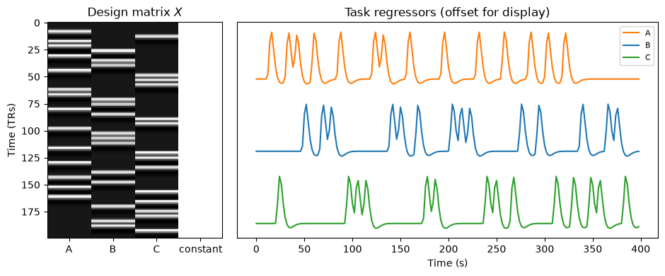

Simulate a voxel and fit the GLM¶

We simulate a voxel that responds most to famous faces, somewhat to non-famous faces, and weakly to houses:

\beta_A = 1.0, \quad \beta_B = 0.6, \quad \beta_C = 0.3, \quad \beta_0 = 100

(1)

β_A, β_B, β_C — true response amplitudes for famous faces, non-famous faces, houses (~% signal change) · β₀ — intercept (baseline signal level)

where $\beta_A$ , $\beta_B$ , and $\beta_C$ are the true response amplitudes for famous faces, non-famous faces, and houses (in ~% signal change), and $\beta_0$ is the intercept — the baseline signal level.

Because each task regressor is peak-normalized to 1 and the intercept is 100, a beta of 1.0 corresponds to roughly a 1% signal change — the units most fMRI papers report.

We fit by ordinary least squares, $\hat{\beta} = (X^TX)^{-1}X^Ty$ , saving the pieces every contrast test will reuse: the residual variance $\hat{\sigma}^2$ , the error degrees of freedom $df_e = n - p$ , and $(X^TX)^{-1}$ .

beta_true = np.array([1.0, 0.6, 0.3, 100.0])   # [A, B, C, intercept]
# Regressors peak at 1 and the intercept is 100, so a beta of 1.0 means a
# 1% signal change; noise SD is 0.15% of baseline.
sigma_noise = 0.15

y = X @ beta_true + sigma_noise * rng.standard_normal(n_scans)

# OLS fit (solve() is more stable than explicitly inverting X'X)
beta_hat = np.linalg.solve(X.T @ X, X.T @ y)

resid = y - X @ beta_hat
n, p = X.shape
dfe = n - p                                     # error degrees of freedom
sigma2_hat = resid @ resid / dfe                # error variance estimate
XtX_inv = np.linalg.inv(X.T @ X)

print(f"dfe = {dfe}, sigma2_hat = {sigma2_hat:.4f} (true {sigma_noise**2:.4f})")
pd.DataFrame({"true beta": beta_true, "estimated beta": beta_hat},
             index=col_names).round(3)

dfe = 196, sigma2_hat = 0.0220 (true 0.0225)

The betas land near their true values. But betas are rarely the final answer — the scientific questions live in comparisons among them.

Step 2 — t-contrasts: one question, one number¶

A contrast is a linear combination of parameters, $c^T\beta$ , chosen so that one scientific question becomes one number. Its estimate is $c^T\hat{\beta}$ , its variance is

\mathrm{Var}(c^T\hat{\beta}) = \sigma^2\, c^T (X^TX)^{-1} c

(2)

Var(c^Tβ̂) — sampling variance of the contrast estimate · c — contrast weight vector · σ² — error variance · X — design matrix (time × predictors)

where $c$ is the contrast weight vector, $\sigma^2$ the error variance, and $X$ the design matrix.

and its t-statistic is

t = \frac{c^T\hat{\beta}}{\sqrt{\hat{\sigma}^2\, c^T (X^TX)^{-1} c}}, \qquad df = df_e

(3)

t — t-statistic for the contrast · c^Tβ̂ — contrast estimate · σ̂² — estimated error variance · df_e — error degrees of freedom (n − p)

where $c^T\hat{\beta}$ is the contrast estimate, $\hat{\sigma}^2$ the estimated error variance, the denominator the contrast’s standard error, and $df_e = n - p$ the error degrees of freedom.

Two rules of thumb:

Comparisons between conditions should use weights that sum to zero (e.g., $[1, -1, 0]$ ), so that $c^T\beta = 0$ under the null hypothesis of equal responses.
Tests against baseline need not sum to zero (e.g., $[1, 0, 0]$ or $[\tfrac13, \tfrac13, \tfrac13]$ ): each $\beta$ is already 0 under the null, so any average of them is too. “Baseline” here means whatever was left unmodeled — the intercept.

Let’s wrap the formula in a function and ask five questions of the same fitted model.

def t_contrast(c, name=""):
    c = np.asarray(c, float)
    value = c @ beta_hat
    se = np.sqrt(sigma2_hat * c @ XtX_inv @ c)
    t = value / se
    return {"contrast": name, "weights [A B C]": np.array2string(c[:3]),
            "true": c @ beta_true, "estimate": value, "SE": se,
            "t": t, "p": 2 * stats.t.sf(abs(t), dfe)}

tests = [
    t_contrast([1, 0, 0, 0],         "A vs. baseline"),
    t_contrast([0, 0, 1, 0],         "C vs. baseline"),
    t_contrast([1, -1, 0, 0],        "A - B (famous - nonfamous)"),
    t_contrast([0.5, 0.5, -1, 0],    "faces - houses"),
    t_contrast([1/3, 1/3, 1/3, 0],   "task average vs. baseline"),
]
pd.DataFrame(tests).set_index("contrast").round(4)

Read the table against the ground truth ( $\beta_A = 1.0$ , $\beta_B = 0.6$ , $\beta_C = 0.3$ ):

Every single-condition and average contrast is strongly positive — this voxel responds to everything relative to baseline.
faces − houses uses $[0.5, 0.5, -1]$ : the positive weights average the two face conditions so the estimate is a difference of means, in the same units as the betas (true value $0.8 - 0.3 = 0.5$ ).
A − B has a smaller t than A vs. baseline even though their SEs are similar: its true effect (0.4) is simply smaller. Notice that the difference contrast’s SE is not larger than the single-condition SEs here — how precisely a design estimates a particular contrast depends on the timing and correlation structure of the regressors (that is design efficiency, Chapter 27).

The same contrast machinery, applied at every voxel, produces the contrast images (COPEs) that carry single-subject effects up to group analysis.

Step 3 — Scaling and centering: interpretation, not inference¶

Scaling contrast weights does not change inference. Multiplying $c$ by any constant scales the estimate and its standard error by the same factor, so t and P are untouched.

for c, name in [([1, -1, 0, 0], "c = [1 -1 0]"),
                ([4, -4, 0, 0], "c = [4 -4 0]")]:
    r = t_contrast(c, name)
    print(f"{name}:  estimate = {r['estimate']:+.3f},  "
          f"t = {r['t']:.3f},  p = {r['p']:.4f}")

c = [1 -1 0]:  estimate = +0.446,  t = 11.425,  p = 0.0000
c = [4 -4 0]:  estimate = +1.783,  t = 11.425,  p = 0.0000

Same t, same p — only the units of the estimate change. Two practical exceptions make the scale worth caring about anyway:

Interpretable units. If you analyze data scaled to percent signal change and want to report contrast values, scale weights so positive weights sum to +1 and negative weights to -1 (e.g., $[0.5, 0.5, -1]$ , not $[1, 1, -2]$ ). Then the contrast is a difference between condition means.
Consistency across participants. Contrast scale must be identical for every subject entering a group analysis. If a participant is missing a run, re-normalize their weights so positives and negatives still sum to $\pm 1$ — otherwise scale differences masquerade as noise (or worse, signal) at the group level.

Centering a covariate changes the intercept’s meaning — nothing else. Suppose we add a continuous covariate $w$ (say, a physiological arousal measure with mean around 3) to the model. Compare fits with raw $w$ versus mean-centered $w$ :

w = 3.0 + rng.standard_normal(n_scans)        # covariate with nonzero mean
y_w = y + 0.5 * w                              # data with a true covariate effect

Xw_raw = np.column_stack([X[:, :3], w, np.ones(n_scans)])
Xw_cen = np.column_stack([X[:, :3], w - w.mean(), np.ones(n_scans)])

b_raw = np.linalg.solve(Xw_raw.T @ Xw_raw, Xw_raw.T @ y_w)
b_cen = np.linalg.solve(Xw_cen.T @ Xw_cen, Xw_cen.T @ y_w)

pd.DataFrame({"uncentered w": b_raw, "centered w": b_cen},
             index=["A", "B", "C", "w (slope)", "intercept"]).round(3)

The task betas and the covariate slope are identical in both fits — so every contrast among them is identical too. Only the intercept moves: with raw $w$ it estimates the expected signal when $w = 0$ (an extrapolation that may be meaningless), while with centered $w$ it estimates the signal at the average covariate value. Centering is about making parameters interpretable, not about changing the model’s fit. The same logic explains why “activation vs. baseline” contrasts always mean “relative to whatever the intercept absorbs.”

Step 4 — F-contrasts: testing several effects jointly¶

A t-contrast tests one linear combination — one degree of freedom, signed. An F-contrast tests whether a set of contrasts is jointly nonzero. Stack the contrasts as rows of a matrix $L$ (each row one contrast, $q$ rows total); then

F = \frac{(L\hat{\beta})^T \left[L (X^TX)^{-1} L^T\right]^{-1} (L\hat{\beta})}{q\, \hat{\sigma}^2} \;\sim\; F_{q,\; df_e} \text{ under } H_0

(4)

F — F-statistic · L — contrast matrix (one contrast per row) · q — number of contrasts (rows) tested · σ̂² — estimated error variance · df_e — error degrees of freedom

where $L$ is the contrast matrix with one contrast per row, $q$ the number of rows (effects tested jointly), $\hat{\sigma}^2$ the estimated error variance, and $df_e$ the error degrees of freedom.

Equivalently, F compares the full model with a reduced model that omits the tested subspace:

F = \frac{(r_0^T r_0 - r^T r)/\nu_1}{r^T r / \nu_2}

(5)

r₀ — reduced-model residuals · r — full-model residuals · ν₁ — number of independent effects tested · ν₂ — error degrees of freedom

where $r_0$ and $r$ are the reduced- and full-model residuals, $\nu_1$ the number of independent effects tested, and $\nu_2$ the error degrees of freedom.

where $r_0$ and $r$ are reduced- and full-model residuals — “how much extra variance do the effects of interest explain?” Typical uses: testing a block of nuisance covariates jointly, an omnibus any-effect test, or testing condition differences across multiple HRF basis functions (whose betas are incommensurate and cannot simply be averaged).

F-tests are unsigned and non-directional: positive and negative deviations both increase F.

def f_contrast(rows):
    L = np.atleast_2d(np.asarray(rows, float))   # one contrast per row
    q = L.shape[0]
    Lb = L @ beta_hat
    F = Lb @ np.linalg.solve(L @ XtX_inv @ L.T, Lb) / (q * sigma2_hat)
    return F, q, stats.f.sf(F, q, dfe)

# 1) Omnibus: does the task explain ANY variance (A, B, C jointly)?
F_any, q, p_any = f_contrast([[1, 0, 0, 0], [0, 1, 0, 0], [0, 0, 1, 0]])
print(f"Any task effect:          F({q},{dfe}) = {F_any:7.2f}, p = {p_any:.3g}")

# ... which equals the full-vs-reduced-model computation (reduced = intercept only)
X0 = np.ones((n_scans, 1))
r0 = y - X0 @ np.linalg.solve(X0.T @ X0, X0.T @ y)
rss0, rss = r0 @ r0, resid @ resid
F_rss = ((rss0 - rss) / 3) / (rss / dfe)
print(f"Full vs. reduced (RSS):   F(3,{dfe}) = {F_rss:7.2f}   <- identical")

# 2) Do the conditions differ from EACH OTHER at all? (one-way ANOVA omnibus)
F_diff, q, p_diff = f_contrast([[1, -1, 0, 0], [0, 1, -1, 0]])
print(f"Any condition difference: F({q},{dfe}) = {F_diff:7.2f}, p = {p_diff:.3g}")

# 3) An F-test of a single contrast is just the square of its t-test
F_ab, _, _ = f_contrast([1, -1, 0, 0])
t_ab = t_contrast([1, -1, 0, 0])["t"]
print(f"F(A-B) = {F_ab:.3f}  =  t(A-B)^2 = {t_ab ** 2:.3f}")

Any task effect:          F(3,196) =  219.15, p = 2.4e-62
Full vs. reduced (RSS):   F(3,196) =  219.15   <- identical
Any condition difference: F(2,196) =  170.76, p = 1.16e-43
F(A-B) = 130.538  =  t(A-B)^2 = 130.538

Three things to notice:

The any-task-effect F is enormous — unsurprising, since all three conditions activate this voxel strongly relative to baseline. The contrast-matrix formula and the full-vs-reduced RSS computation agree exactly: they are the same test.
The any-condition-difference F spans just two rows ( $A-B$ and $B-C$ ), yet those two rows span all pairwise differences — including $A-C$ , which is their sum. It ignores the (huge) shared activation vs. baseline and asks only whether the conditions differ from each other.
A one-row F-contrast reproduces the two-tailed t-test, with $F = t^2$ — but it discards the sign.

Step 5 — Conjunction: “A and B”, not “A or B”¶

An F-test asks whether any combination of the tested effects is nonzero — a logical OR (and an unsigned one). Many scientific claims are logical AND claims: for instance, “this region responds to faces whether or not they are famous” requires both $A - C > 0$ and $B - C > 0$ .

The simple, valid way to test the AND claim (the conjunction null) is the minimum-statistic rule: declare a conjunction only if every component contrast individually exceeds the significance threshold — equivalently, if $\min(t_1, t_2) > t_{crit}$ . Beware the common fallacy of concluding “both effects present” from a significant F or from one significant test plus one non-significant test.

We simulate two new voxels with the same design:

Voxel 1 responds to both face types ( $\beta = [0.9, 0.8, 0.1]$ ) — a genuinely face-selective region
Voxel 2 responds only to famous faces ( $\beta = [0.9, 0.1, 0.1]$ )

def voxel_contrast_tests(beta_v, label):
    y_v = X @ beta_v + sigma_noise * rng.standard_normal(n_scans)
    b = np.linalg.solve(X.T @ X, X.T @ y_v)
    r = y_v - X @ b
    s2 = r @ r / dfe
    out = {"voxel": label}
    for name, c in [("A-C", [1, 0, -1, 0]), ("B-C", [0, 1, -1, 0])]:
        c = np.asarray(c, float)
        out[f"t({name})"] = c @ b / np.sqrt(s2 * c @ XtX_inv @ c)
    out["min t"] = min(out["t(A-C)"], out["t(B-C)"])
    return out

t_crit = stats.t.ppf(0.95, dfe)                # one-sided, alpha = .05
print(f"t_crit (one-sided, alpha = .05, df = {dfe}) = {t_crit:.2f}\n")

conj = pd.DataFrame([
    voxel_contrast_tests(np.array([0.9, 0.8, 0.1, 100.0]), "1: A and B > houses"),
    voxel_contrast_tests(np.array([0.9, 0.1, 0.1, 100.0]), "2: only A > houses"),
]).set_index("voxel")
conj["conjunction?"] = conj["min t"] > t_crit
conj.round(2)

t_crit (one-sided, alpha = .05, df = 196) = 1.65

Voxel 1 passes the conjunction — both contrasts clear the threshold on their own, so we can claim the region responds to famous and non-famous faces more than houses. Voxel 2 shows a strong famous-face effect, but its $t(B{-}C)$ hovers near zero, the minimum statistic fails, and the AND claim is (correctly) rejected — even though an F-test over the same two contrasts would light up brightly for this voxel. Choosing between F (any effect) and conjunction (all effects) is choosing which logical question you are asking.

Where to go next¶

Chapter 21: contrast images computed here become the inputs to group-level (second-level) analysis
Chapter 22: running these tests at ~100,000 voxels demands multiple-comparisons correction
Chapter 19: with real fMRI noise, replace $\hat{\sigma}^2 (X^TX)^{-1}$ with its GLS/prewhitened counterpart — the contrast logic is unchanged

Exercises

Test the contrast $[1, -0.5, -0.5, 0]$ (“famous faces vs. the average of everything else”). What is its true value under our simulation? Verify your prediction.
The weights $[2, -1, -1, 0]$ and $[1, -0.5, -0.5, 0]$ test the same hypothesis. Confirm the t-values match, then state which scaling you would report for percent-signal-change data and why.
Build the 2×2 factorial from the chapter (conditions A–D) by splitting each of our three conditions differently: simulate four conditions with betas $[1.0, 0.8, 0.5, 0.7]$ and test the two main effects and the interaction using $[1, 1, -1, -1]$ , $[1, -1, 1, -1]$ , and $[1, -1, -1, 1]$ (each with a 0 for the intercept). Which effects are detectable?
In the conjunction demo, gradually raise voxel 2’s $\beta_B$ from 0.1 toward 0.8 (re-running the simulation several times per value). Around what effect size does the conjunction start to succeed reliably? What does this tell you about the power cost of AND claims?