The General Linear Model and Foundations of Analysis
Run this code: ⚡ In-browser lab · Colab · MATLAB Online
Overview
The General Linear Model is arguably the most widely used statistical method for relating task manipulations to brain activity. Applied to fMRI, it identifies regions that respond to an event type, compares responses across conditions, and links brain activity to behavioral or clinical variables. In a typical analysis the outcome variable is the time series from a single voxel (or region of interest), and the analysis is massively univariate: a separate GLM is fit at every voxel, and the resulting parameter estimates are assembled into statistical maps.
The GLM is really a family of models in which one continuously distributed outcome () is predicted by a linear combination of predictors (the columns of a design matrix ). This family includes t-tests, multiple regression, ANOVA, and ANCOVA — the number, distribution, and grouping of predictors determines which label applies. GLMs have three big advantages: they have a closed-form solution so estimation is fast and reproducible; they are easy to interpret; and they are flexible, since nonlinear relationships can be captured with transformed predictors, piecewise terms, or splines. Extensions handle situations where the basic assumptions fail: generalized least squares for correlated or unequal-variance errors, linear mixed models for grouped observations such as participants, and generalized linear models (via link functions) for binary or count outcomes.
Modeling task-evoked BOLD signal begins with two ingredients: a neural stimulus function describing when neural activity is assumed to occur — brief events or sustained epochs (blocks) — and a hemodynamic response function describing the sluggish vascular response to a burst of neural activity. Assuming the brain behaves as a linear time invariant (LTI) system, the predicted signal is the convolution of the two:
x(t) — predicted BOLD signal · s(t) — neural stimulus function (1 during assumed activity, 0 elsewhere) · h(t) — hemodynamic response function · ∗ — convolution
where is the predicted BOLD signal, the neural stimulus function, the hemodynamic response function, and the convolution operator.
LTI systems have three key properties: scaling (doubling neural activity doubles the BOLD response, so amplitude differences between conditions can be interpreted as neural differences), superposition (responses to nearby events sum), and time invariance (shifting a stimulus shifts its response). Linearity is a good approximation when events are spaced at least ~5 seconds apart, though nonlinearities (e.g., refractory effects) can be substantial for stimuli spaced under ~2 seconds.
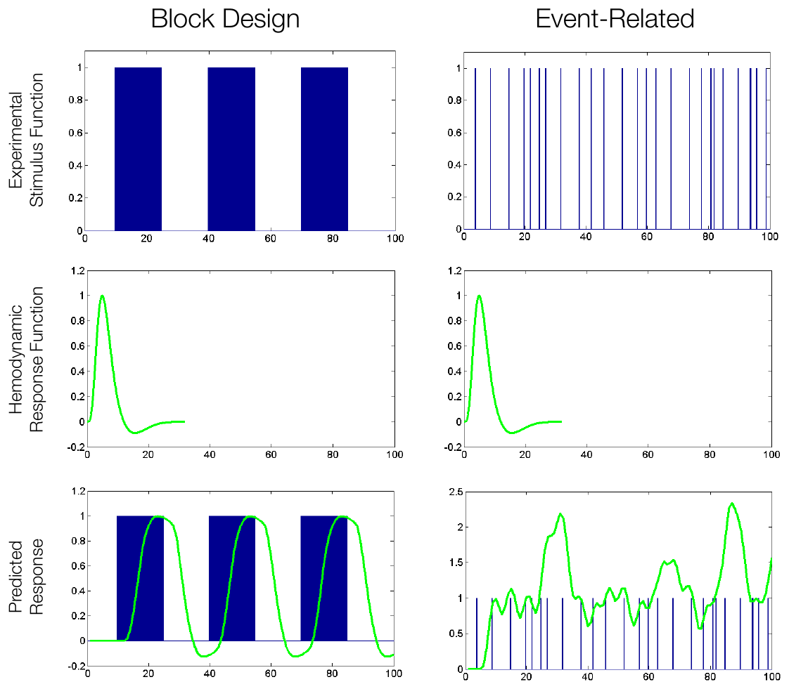
The linear system framework used in fMRI. An experimental stimulus function — a block design (left) or event-related design (right) — is convolved with a canonical HRF to obtain the predicted BOLD response. (Figure 18.2 from the book. © the authors and MIT Press; reproduced with permission — not covered by this site’s CC-BY license.)
A popular canonical HRF is the difference of two gamma functions, which captures the initial peak around 5–6 seconds and the subsequent undershoot:
h(t) — HRF value at time t after a neural event · α₁, β₁ — shape and rate of the peak gamma · α₂, β₂ — shape and rate of the undershoot gamma · c — undershoot amplitude · Γ — gamma function
where is time since the neural event, are the shape and rate parameters of the first (peak) gamma function, those of the second (undershoot) gamma, scales the undershoot, and is the gamma function.
with common choices , , , and .
To formulate the GLM, each condition’s indicator vector (1 during hypothesized neural activity, 0 elsewhere) is convolved with the HRF, and the resulting predicted time courses become columns of the design matrix , alongside an intercept and any nuisance covariates (head motion estimates, drift terms). With time points and predictors, the model is
y — voxel time series (n × 1) · X — design matrix (n × p) · β — unknown amplitudes (p × 1) · ε — unexplained error, variance σ² · I — identity matrix
where is the voxel time series, the design matrix, a vector of unknown amplitudes, the vector of unexplained errors with variance , and the identity matrix.
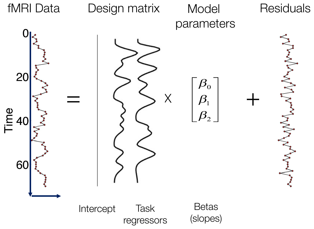
A pictorial representation of the standard GLM setup. The fMRI time series from one voxel (left) is modeled as the design matrix — here an intercept plus two task regressors — multiplied by three beta values, plus residuals. (Figure 18.3 from the book. © the authors and MIT Press; reproduced with permission — not covered by this site’s CC-BY license.)
Estimation seeks the values that minimize the sum of squared errors . A closed-form solution exists — the ordinary least squares (OLS) estimate:
β̂ — estimated coefficients · X — design matrix (time × predictors) · y — voxel time series · ᵀ — transpose
where is the vector of estimated coefficients, the design matrix, the measured time series, and the transpose operator.
with error variance estimated from the residuals as . Under the model assumptions, is the best linear unbiased estimate (BLUE), distributed as .
Inference on each compares it with a null value of zero. Its standard error is the square root of the th diagonal of , and the ratio follows a Student’s t distribution with error degrees of freedom. A low P value lets us declare a region activated () or deactivated () — always relative to the model’s intercept, which reflects unmodeled baseline periods. The same machinery extends to contrasts across conditions (Chapter 20).
Two refinements matter in practice. First, fMRI errors are not independent — they are autocorrelated — so OLS standard errors are too small and t-statistics inflated. The remedy is generalized least squares (GLS): assume a structured error covariance and prewhiten, giving , with and estimated iteratively (Chapter 19). Second, the canonical HRF’s shape varies across brain regions and individuals, and mis-modeling it reduces power and can produce false positives. Basis sets — such as the canonical HRF plus temporal and dispersion derivatives, or the highly flexible finite impulse response (FIR) model with one parameter per post-stimulus time point — let the fitted response adapt, at the cost of a fundamental tradeoff between flexibility and power: too much flexibility risks fitting noise.
Hands-on tutorial
In this tutorial you will build a design matrix from event onsets and fit a GLM to a simulated voxel time series — the core of every first-level fMRI analysis. The figure below shows the recipe: indicator functions marking event onsets are convolved with an assumed HRF, and the resulting predictors become columns of .
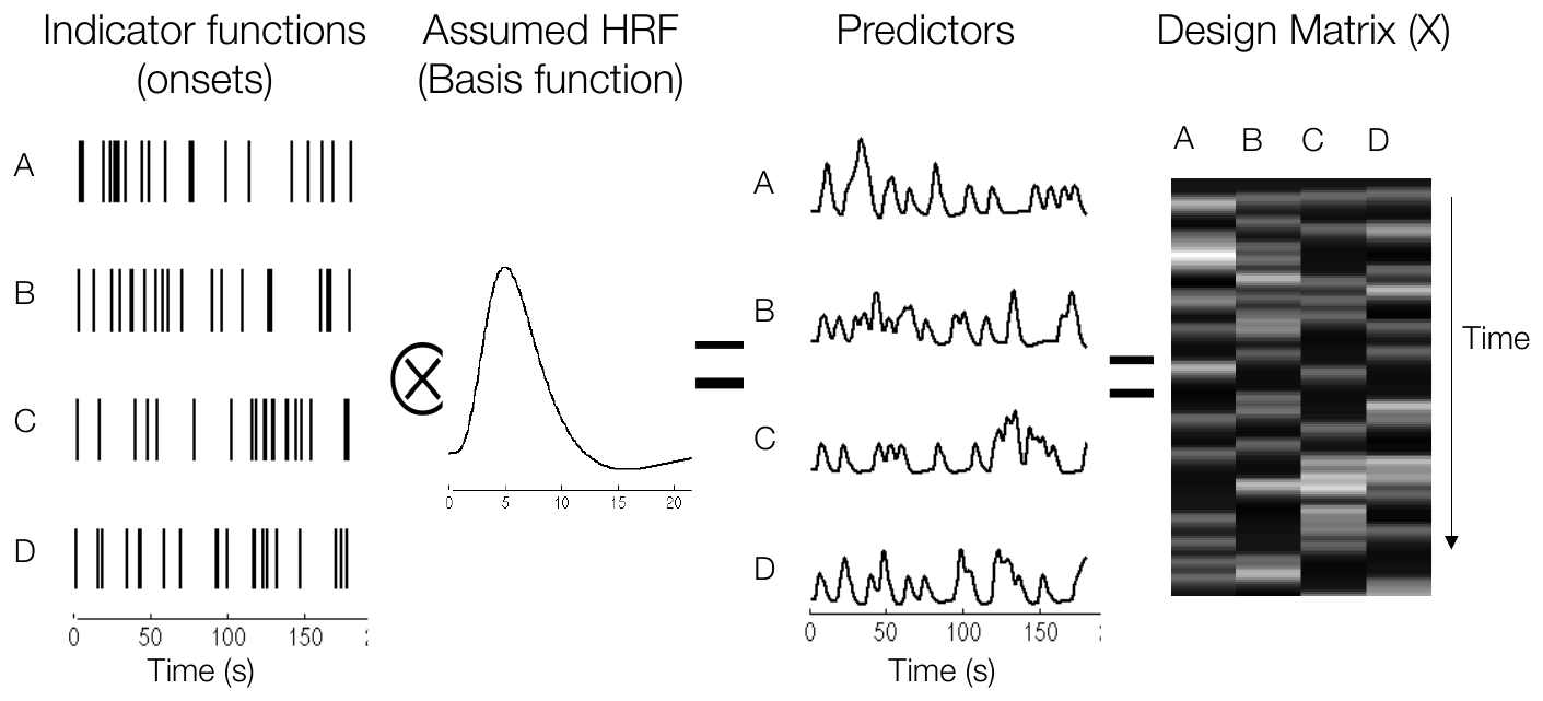
Creating a design matrix with four conditions. Indicator functions for the timing of conditions A–D are convolved with a canonical HRF to obtain four predicted responses, which become columns of the design matrix. (Figure 18.4 from the book. © the authors and MIT Press; reproduced with permission — not covered by this site’s CC-BY license.)
Step 1 — Build a design matrix from event onsets. We specify onset times (in seconds) for two event types, A and B, and convolve them with a canonical HRF.
% Requires CanlabCore + SPM12 on your MATLAB path
% Adapted from CANlab tutorials (github.com/canlab)
TR = 2;                                       % repetition time (s)
n_scans = 180;                                % number of volumes (6-min run)

ons = {};
ons{1} = [10 60 110 160 210 260 310]';        % Condition A onsets (sec)
ons{2} = [35 85 135 185 235 285 335]';        % Condition B onsets (sec)

% Convolve onsets with canonical HRF; intercept is the last column
X = onsets2fmridesign(ons, TR, n_scans * TR);

plotDesign(ons, [], TR);                       % plot regressors and onsets
figure; imagesc(X); colormap gray;             % view X as an image
xlabel('Regressor'); ylabel('Time (TRs)');
import numpy as np, pandas as pd
from nilearn.glm.first_level import make_first_level_design_matrix
from nilearn.plotting import plot_design_matrix
t_r, n_scans = 2.0, 180 # t_r = repetition time (s); n_scans = volumes (6-min run)
frame_times = np.arange(n_scans) * t_r
events = pd.DataFrame({
"onset": [10, 60, 110, 160, 210, 260, 310, # Condition A
35, 85, 135, 185, 235, 285, 335], # Condition B
"duration": [1.0] * 14, # every event lasts 1 s
"trial_type": ["A"] * 7 + ["B"] * 7,
})
# Convolve onsets with canonical HRF; 'constant' (intercept) is last column
X = make_first_level_design_matrix(frame_times, events,
hrf_model="spm", drift_model=None)
plot_design_matrix(X) # view X as an imageExample output: running the Python tab draws the classic design-matrix image — 180 rows (one per volume) by 3 columns (regressors A and B, plus the constant/intercept):
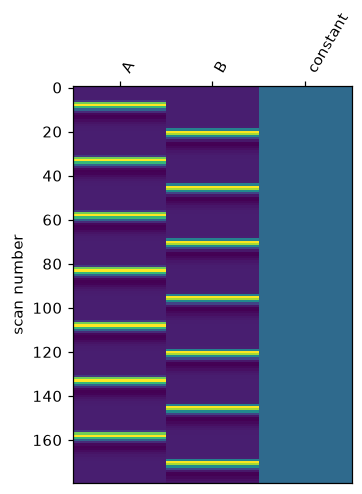
The design matrix as an image: one row per volume, one column per regressor. Each bright band is the HRF-convolved response to one event. The MATLAB tab’s imagesc(X) view is analogous.
Step 2 — Fit the GLM to a voxel time series. We simulate a voxel with known true effects (, , intercept 100) plus modest Gaussian noise (, where is the noise standard deviation) and recover them with the OLS formula .
% Simulate a voxel: y = X * beta_true + noise
rng(9);                                        % seed for reproducible noise
beta_true = [0.8 0.4 100]';                    % true effects: A, B, intercept (last col)
sigma_noise = 0.5;                             % noise SD; modest so this short 7-event demo recovers betas clearly
y = X * beta_true + sigma_noise * randn(n_scans, 1);

% Ordinary least squares: beta_hat = (X'X)^{-1} X'y
beta_hat = (X' * X) \ (X' * y);

r      = y - X * beta_hat;                     % residuals
dfe    = n_scans - size(X, 2);                 % error degrees of freedom (n - p)
sigma2 = (r' * r) / dfe;                       % error variance estimate
t_vals = beta_hat ./ sqrt(sigma2 * diag(inv(X' * X)));

disp(table(beta_true, beta_hat, t_vals))
# Simulate a voxel: y = X @ beta_true + noise
Xm = X.to_numpy().copy() # design as array; columns: A, B, constant
Xm[:, :2] /= Xm[:, :2].max(axis=0) # rescale task regressors to unit peak, so betas are in signal units
rng = np.random.default_rng(1) # seed for reproducible noise
beta_true = np.array([0.8, 0.4, 100.0]) # true effects: A, B, intercept
sigma_noise = 0.5 # noise SD; modest so this short 7-event demo recovers betas clearly
y = Xm @ beta_true + sigma_noise * rng.standard_normal(n_scans)
# Ordinary least squares: beta_hat = (X'X)^{-1} X'y
beta_hat = np.linalg.solve(Xm.T @ Xm, Xm.T @ y)
resid = y - Xm @ beta_hat # residuals
dfe = n_scans - Xm.shape[1] # error degrees of freedom (n - p)
sigma2 = resid @ resid / dfe # error variance estimate
t_vals = beta_hat / np.sqrt(sigma2 * np.diag(np.linalg.inv(Xm.T @ Xm)))
print(pd.DataFrame({"true": beta_true, "estimate": beta_hat, "t": t_vals},
index=X.columns))Example output: the Python tab prints the recovered parameters — close to the true values, with clear t-statistics for both conditions (the MATLAB tab produces an analogous table):
           true   estimate            t
A           0.8   0.787951     6.314865
B           0.4   0.399651     3.223820
constant  100.0  99.964533  2647.254402
The estimates land close to the true values, with reliable t-statistics for both conditions. The full labs continue the arc: inspecting residuals and model fit (), computing standard errors and P values, and testing a simple A − B contrast — the bridge to Chapter 20.
Open the full Python lab notebook → or download the MATLAB live script, which mirrors it using CANlab tools.
Thought questions
Suppose your experiment presents stimuli in rapid sequences, spaced 1–2 seconds apart. Which LTI assumptions are most at risk, how might your estimates be distorted, and what design or modeling choices could mitigate the problem?
The HRF varies across brain regions and individuals — for instance, patients with vascular disease may show delayed or blunted responses. If you compare patients and controls using a fixed canonical HRF, how could HRF mis-modeling masquerade as group differences in “activation”?
Adding nuisance regressors (motion, drift) can both improve and worsen your inferences. Using the concepts of residual variance and error degrees of freedom, explain when each outcome would occur.
Activation in the GLM is always relative to the intercept (baseline). How does your choice of what to leave unmodeled change the interpretation of a significant positive beta? Give a concrete example where two labs modeling the same data differently would reach different verbal conclusions.
The FIR basis set can fit almost any response shape, yet most researchers use a single canonical HRF. Drawing on the power–flexibility tradeoff, when would you recommend each approach, and what would you look at in the data to decide?
Quiz yourself
Q1. In a single-subject fMRI GLM, what is the outcome variable , and what does “massively univariate” mean?
Answer: is the BOLD time series from a single voxel (or region of interest). “Massively univariate” means a separate GLM is fit independently at every voxel in the brain, and the results are assembled into statistical maps.
Q2. What two ingredients are combined — and by what mathematical operation — to create a task predictor for the design matrix?
Answer: A stimulus (indicator) function coding when neural activity is assumed to occur is convolved with a hemodynamic response function (HRF). The convolution gives the predicted BOLD time course, which becomes a column of .
Q3. Name and briefly define the three properties of a linear time invariant (LTI) system.
Answer: Scaling: multiplying the input by a factor scales the response by the same factor. Superposition: the response to two stimuli together is the sum of their individual responses. Time invariance: shifting a stimulus in time shifts its response by the same amount.
Q4. What is the OLS estimate of , and what optimality property does it have when errors are independent and identically distributed?
Answer: . Under IID errors it is the best linear unbiased estimate (BLUE): among all linear unbiased estimators, it has the smallest variance.
Q5. With time points and predictors (including the intercept), what are the error degrees of freedom, and why do they matter?
Answer: . The error degrees of freedom determine how precisely the error variance is estimated, and they define the t distribution used to compute P values — fewer means less certainty and wider tails.
Q6. Why does plain OLS give invalid inferences for fMRI time series, and what is the standard remedy?
Answer: fMRI errors are autocorrelated (and can be heteroskedastic), violating the independence assumption. As a result the variance of is underestimated, t-statistics are inflated, and P values are too liberal. The remedy is generalized least squares: model the error covariance , prewhiten, and estimate , iterating between estimates of and .
Q7. What is the finite impulse response (FIR) basis set, and what is its main advantage and main risk?
Answer: The FIR model includes one free parameter for each time point following stimulus onset, so the estimated betas trace out the average response shape with minimal assumptions. Its advantage is flexibility to capture HRF variation; its risk is overfitting — modeling noise as well as signal — which produces noisier, less generalizable estimates.
 The book: Elements of Functional Magnetic Resonance Imaging — Wager & Lindquist, MIT Press