This lab accompanies Chapter 17, “Image Preprocessing”. Real preprocessing runs inside packages like SPM, FSL, and fMRIPrep — here we simulate the concepts behind four key steps so you can see exactly what each one fixes and what it costs: (1) head motion and nuisance regression, (2) slice-timing offsets, (3) smoothing-kernel tradeoffs, and (4) high-pass filter design for drift removal.
How to run this notebook: it uses only numpy, scipy, and matplotlib on simulated data, so it runs in the browser (JupyterLite/Pyodide), on Colab, or locally. Each cell takes at most a few seconds. Run cells top to bottom. See the chapter page for the concepts.
▶ This notebook is interactive. Click the ⏻ power icon at the top right of this page to run it in your browser — no installation needed (the kernel takes ~30–60 s to start the first time). Then run cells top to bottom, starting with the first code cell below: later cells depend on the imports and variables defined earlier, and will error if you skip ahead.
import numpy as np
import matplotlib.pyplot as plt
from scipy import ndimage, signal
from scipy.linalg import pinv

rng = np.random.default_rng(17)
plt.rcParams.update({"figure.figsize": (9, 4), "axes.spines.top": False,
                     "axes.spines.right": False})
Lab 1 — Head motion: realignment parameters as nuisance regressors
Realignment estimates six rigid-body parameters per volume: translations in (mm) and rotations roll, pitch, yaw (radians). These parameter time courses are saved by every preprocessing package (e.g., SPM’s rp_*.txt files) and are routinely included as nuisance covariates in the GLM.
We simulate a 200-volume run (TR = 1 s) in which the head drifts slowly (a random walk) and makes one sudden jerk. The voxel’s signal is a mix of “neural” fluctuations, motion-coupled artifact, and thermal noise — so we know exactly how much variance motion is responsible for, and we can check how much of it the realignment parameters recover.
n, TR = 200, 1.0   # n = volumes (frames); TR = repetition time (s)

# --- Six motion parameters: slow random-walk drift + one sudden jerk
mp = np.cumsum(0.02 * rng.standard_normal((n, 6)), axis=0)
mp[:, 3:] *= 0.005                      # rotations are small (radians)
mp[120:125, :3] += 0.8                  # 0.8 mm translation jerk at frame 120
mp[120:125, 3:] += 0.004                # with a small rotation component

# --- Voxel time series: neural signal + motion-coupled artifact + noise
neural = signal.lfilter([1.0], [1.0, -0.5, -0.1], rng.standard_normal(n))  # AR(2) fluctuations
motion_weights = np.array([2.0, 1.5, 1.0, 300.0, 200.0, 100.0])  # coupling of each param to this voxel
motion_artifact = mp @ motion_weights
y = neural + motion_artifact + 0.5 * rng.standard_normal(n)

fig, axes = plt.subplots(2, 1, figsize=(9, 5), sharex=True)
axes[0].plot(mp[:, :3])
axes[0].set_ylabel("Translation (mm)"); axes[0].legend(["x", "y", "z"], loc="upper left")
axes[0].set_title("Simulated realignment parameters")
axes[1].plot(np.degrees(mp[:, 3:]))
axes[1].set_ylabel("Rotation (deg)"); axes[1].set_xlabel("Frame")
axes[1].legend(["pitch", "roll", "yaw"], loc="upper left")
plt.tight_layout()
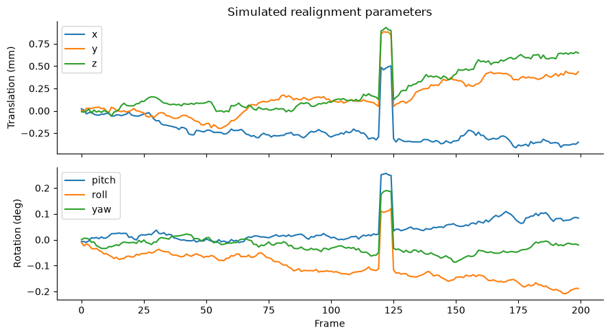
These traces are what you should always plot for every run you preprocess (compare Figure 17.3 in the book). Slow drifts are normal; sudden steps like the one at frame 120 are the dangerous ones.
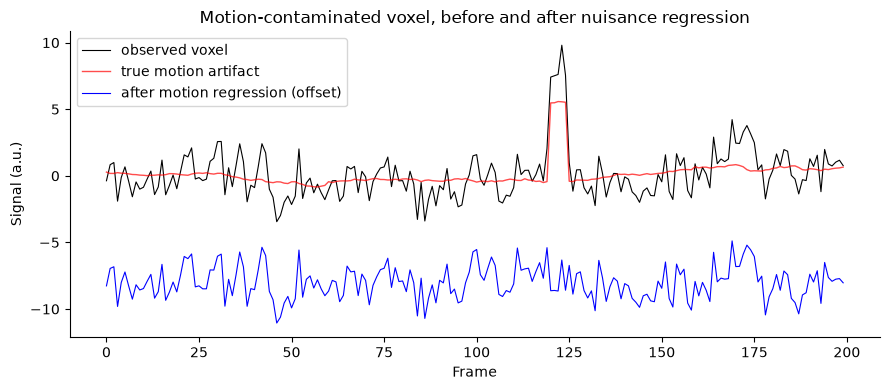
How much voxel variance does motion explain? We regress the voxel on the six parameters (plus an intercept) and compute — the fraction of variance the realignment parameters account for.
X = np.column_stack([mp, np.ones(n)])
beta = np.linalg.lstsq(X, y, rcond=None)[0]
resid = y - X @ beta
r2_motion = 1 - resid.var() / y.var()
print(f"Variance explained by the 6 motion parameters: R^2 = {r2_motion:.2f}")

fig, ax = plt.subplots()
ax.plot(y, "k", lw=0.8, label="observed voxel")
ax.plot(motion_artifact + y.mean() - motion_artifact.mean(), "r", lw=1,
        alpha=0.7, label="true motion artifact")
ax.plot(resid - 8, "b", lw=0.8, label="after motion regression (offset)")
ax.set_xlabel("Frame"); ax.set_ylabel("Signal (a.u.)"); ax.legend(loc="upper left")
ax.set_title("Motion-contaminated voxel, before and after nuisance regression")
plt.tight_layout()
Variance explained by the 6 motion parameters: R^2 = 0.56
Framewise displacement and censoring. FWD summarizes the six parameters into one number per frame: the sum of absolute frame-to-frame changes, with rotations converted to millimeters as arc length on a 50-mm-radius sphere,
FWDₜ — framewise displacement at frame t (mm) · Δd — frame-to-frame change in each translation (mm) · Δα, Δβ, Δγ — changes in the three rotations (radians) · 50 — sphere radius (mm) converting rotation to arc length
where is the framewise displacement at frame , are the frame-to-frame changes in the three translations (mm), the changes in the three rotations (radians), and 50 mm is the sphere radius used to convert rotations to arc length.
Frames exceeding a threshold (0.2–0.5 mm is typical) are censored — preferably by spike regression: one extra nuisance regressor per bad frame, which zeroes out that frame’s influence while preserving the temporal structure of the rest of the series.
fwd = (np.abs(np.diff(mp[:, :3], axis=0)).sum(axis=1)
       + 50 * np.abs(np.diff(mp[:, 3:], axis=0)).sum(axis=1))
fwd = np.r_[0, fwd]                      # first frame has no predecessor
thresh = 0.5                             # censoring threshold (mm); 0.2-0.5 mm is typical
bad = np.where(fwd > thresh)[0]
print(f"Mean FWD = {fwd.mean():.3f} mm; {bad.size} frames exceed {thresh} mm: {bad}")

# Spike regressors: one indicator column per censored frame
spikes = np.zeros((n, bad.size))
spikes[bad, np.arange(bad.size)] = 1

X2 = np.column_stack([mp, spikes, np.ones(n)])
resid2 = y - X2 @ np.linalg.lstsq(X2, y, rcond=None)[0]
print(f"R^2, motion params only:          {r2_motion:.3f}")
print(f"R^2, motion params + spike regs:  {1 - resid2.var() / y.var():.3f}")

fig, ax = plt.subplots()
ax.plot(fwd, "k")
ax.axhline(thresh, color="r", ls="--", label=f"censoring threshold ({thresh} mm)")
ax.plot(bad, fwd[bad], "rv", label="censored frames")
ax.set_xlabel("Frame"); ax.set_ylabel("FWD (mm)"); ax.legend()
ax.set_title("Framewise displacement")
plt.tight_layout()
Mean FWD = 0.089 mm; 2 frames exceed 0.5 mm: [120 125]
R^2, motion params only:          0.563
R^2, motion params + spike regs:  0.566
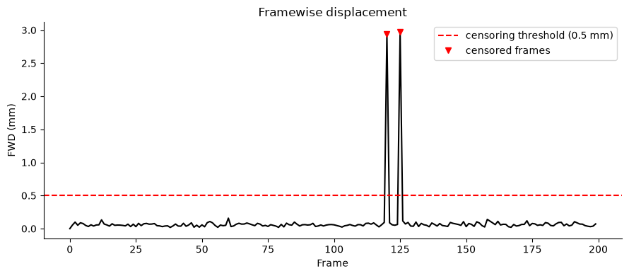
Interpretation. The six realignment parameters soak up most of the motion-related variance, and spike regressors mop up the residual effect of the jerk. In real data motion also leaves spin-history artifacts that realignment cannot fix — which is why prevention (padding, coaching, tactile feedback) plus conservative censoring beats aggressive exclusion. Remember the selection-bias warning from the chapter: motion correlates with age, BMI, and clinical status, so excluding many participants for motion can bias your sample.
Lab 2 — Slice-timing offsets and interpolation
Slices are acquired at different moments within each TR, but analysis treats each volume as a snapshot. With TR = 2 s and 20 slices acquired interleaved (odd slices first, then even), two anatomically adjacent slices can be sampled almost a full second apart.
We simulate a “true” continuous BOLD response shared by voxels in three slices — bottom (slice 0), middle (slice 10), and top (slice 19) — and sample each voxel at its actual acquisition times. Then we apply slice-timing correction by interpolating every series to the reference slice’s acquisition times.
def double_gamma_hrf(t, a1=6, a2=16, b1=1, b2=1, c=1/6):
    """Canonical double-gamma HRF evaluated at times t (s)."""
    from scipy.special import gamma as G
    h = (t**(a1-1) * b1**a1 * np.exp(-b1*t) / G(a1)
         - c * t**(a2-1) * b2**a2 * np.exp(-b2*t) / G(a2))
    h[t < 0] = 0
    return h

TR, n_vol, n_slices = 2.0, 100, 20  # TR (s); volumes; slices per volume
dt = 0.05                           # high-resolution time step (s)
t_hi = np.arange(0, n_vol * TR, dt)

# Continuous BOLD: events every 24 s convolved with the HRF
onsets = np.arange(6, n_vol * TR - 20, 24)   # one event every 24 s
stim = np.zeros_like(t_hi)
stim[(onsets / dt).astype(int)] = 1
bold = np.convolve(stim, double_gamma_hrf(np.arange(0, 32, dt)))[:t_hi.size]

# Interleaved acquisition order: slices 0,2,4,...,1,3,5,...
order = np.r_[np.arange(0, n_slices, 2), np.arange(1, n_slices, 2)]
slice_offset = np.empty(n_slices)
slice_offset[order] = np.arange(n_slices) * (TR / n_slices)

# Sample each slice's voxel at its true acquisition times
vol_times = np.arange(n_vol) * TR
picks = {"slice 0 (first)": 0, "slice 10 (middle)": 10, "slice 19 (last)": 19}
sampled = {name: np.interp(vol_times + slice_offset[s], t_hi, bold)
           for name, s in picks.items()}
for name, s in picks.items():
    print(f"{name}: acquired {slice_offset[s]:.2f} s into each TR")
slice 0 (first): acquired 0.00 s into each TR
slice 10 (middle): acquired 0.50 s into each TR
slice 19 (last): acquired 1.90 s into each TR
ref_slice = 10                                   # reference: middle of the TR
ref_offset = slice_offset[ref_slice]

fig, axes = plt.subplots(2, 1, figsize=(9, 6), sharex=True)
axes[0].plot(t_hi, bold, "k", lw=0.8, alpha=0.5, label="true continuous BOLD")
for name, s in picks.items():
    axes[0].plot(vol_times, sampled[name], "o-", ms=3, lw=0.8, label=name)
axes[0].set_xlim(0, 60); axes[0].legend(fontsize=8)
axes[0].set_title("Uncorrected: same response, sampled at different slice times")

# Slice-timing correction: interpolate each series to the reference times
for name, s in picks.items():
    corrected = np.interp(vol_times + ref_offset,
                          vol_times + slice_offset[s], sampled[name])
    axes[1].plot(vol_times, corrected, "o-", ms=3, lw=0.8, label=name)
axes[1].plot(t_hi, bold, "k", lw=0.8, alpha=0.5)
axes[1].set_xlim(0, 60); axes[1].legend(fontsize=8)
axes[1].set_xlabel("Time (s)")
axes[1].set_title(f"After slice-timing correction to slice {ref_slice}")
plt.tight_layout()
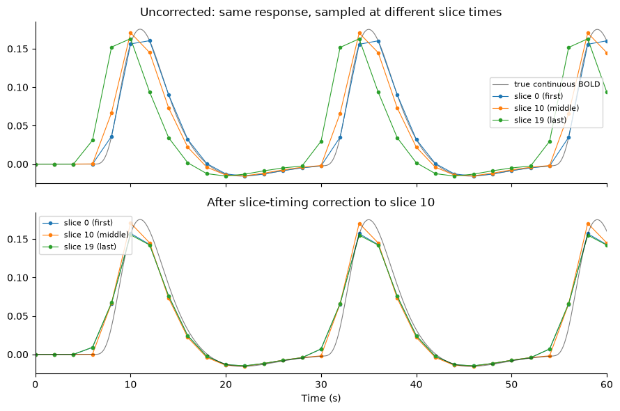
Why the offsets matter for estimation. Suppose we fit each voxel with a canonical regressor built for the reference slice’s timing. For a mistimed voxel, the regressor is shifted relative to the data, so the estimated amplitude (beta) is biased downward — signal leaks into the residuals.
# Canonical regressor built at the reference slice's timing
regressor = np.interp(vol_times + ref_offset, t_hi, bold)
regressor = (regressor - regressor.mean()) / regressor.std()

print(f"{'voxel':<20}{'beta, uncorrected':>20}{'beta, corrected':>20}")
for name, s in picks.items():
    yv = sampled[name]
    corrected = np.interp(vol_times + ref_offset,
                          vol_times + slice_offset[s], yv)
    for label, data in [("unc", yv), ("cor", corrected)]:
        d = data - data.mean()
        b = (regressor @ d) / (regressor @ regressor)
        if label == "unc":
            b_unc = b
        else:
            print(f"{name:<20}{b_unc:>20.3f}{b:>20.3f}")
voxel                  beta, uncorrected     beta, corrected
slice 0 (first)                    0.060               0.058
slice 10 (middle)                  0.061               0.061
slice 19 (last)                    0.053               0.058
Interpretation. With interleaved acquisition and TR = 2 s, the last-acquired slice is sampled ~1.9 s later than the first — enough to shift the sampled response visibly and bias amplitude estimates. Interpolation to a reference slice fixes most of it, at the cost of some interpolation error (and it can smear spikes and interact with motion). With TR ≤ 1 s, timing offsets shrink and many pipelines skip this step, instead shifting task regressors per slice or using flexible basis sets — the option recommended in the chapter for rapid acquisitions.
Lab 3 — Smoothing kernel tradeoffs: the matched filter
Smoothing convolves the image with a 3-D Gaussian kernel described by its FWHM (, where is the standard deviation of the Gaussian kernel). Matched-filter theory says detection is optimal when the kernel matches the spatial extent of the signal: smooth too little and voxel noise dominates; smooth too much and you average true signal with null neighbors (partial-volume dilution).
We simulate a 2-D “brain slice” (2-mm voxels) with two activation blobs — one small (FWHM ≈ 7 mm) and one large (FWHM ≈ 28 mm), equal peak amplitude — plus voxelwise noise, and measure detection strength (peak z at the blob center) as a function of smoothing FWHM.
vox_mm = 2.0   # voxel size (mm)
size = 100     # image grid size (voxels per side)
yy, xx = np.mgrid[0:size, 0:size]

def gauss_blob(cx, cy, sigma_vox, amp=1.0):
    return amp * np.exp(-((xx - cx)**2 + (yy - cy)**2) / (2 * sigma_vox**2))

sigma_small, sigma_large = 1.5, 6.0            # in voxels
truth = (gauss_blob(28, 50, sigma_small) + gauss_blob(70, 50, sigma_large))
print(f"small blob FWHM ~ {2.355 * sigma_small * vox_mm:.0f} mm, "
      f"large blob FWHM ~ {2.355 * sigma_large * vox_mm:.0f} mm")

noise_sd = 1.0                                 # voxelwise noise SD
fwhms_mm = np.arange(0, 17, 1)                  # smoothing kernels to test
n_sims = 60                                    # noise realizations per kernel

z_small, z_large = [], []
for fwhm in fwhms_mm:
    sigma_vox = fwhm / 2.355 / vox_mm
    peaks_s, peaks_l, noise_sds = [], [], []
    for _ in range(n_sims):
        img = truth + noise_sd * rng.standard_normal((size, size))
        sm = ndimage.gaussian_filter(img, sigma_vox) if sigma_vox > 0 else img
        peaks_s.append(sm[50, 28]); peaks_l.append(sm[50, 70])
        noise_sds.append(sm[5:20, 5:20].std())   # background patch
    sd = np.mean(noise_sds)
    z_small.append(np.mean(peaks_s) / sd)
    z_large.append(np.mean(peaks_l) / sd)
z_small, z_large = np.array(z_small), np.array(z_large)
small blob FWHM ~ 7 mm, large blob FWHM ~ 28 mm
fig, axes = plt.subplots(1, 4, figsize=(11, 3))
img = truth + noise_sd * rng.standard_normal((size, size))
for ax, fwhm in zip(axes, [0, 4, 8, 16]):
    sigma_vox = fwhm / 2.355 / vox_mm
    sm = ndimage.gaussian_filter(img, sigma_vox) if sigma_vox > 0 else img
    ax.imshow(sm, cmap="gray"); ax.set_title(f"FWHM = {fwhm} mm", fontsize=9)
    ax.axis("off")
plt.suptitle("Small (left blob) and large (right blob) activations under smoothing")
plt.tight_layout()

fig, ax = plt.subplots(figsize=(7, 4))
ax.plot(fwhms_mm, z_small, "o-", label=f"small blob (~7 mm)")
ax.plot(fwhms_mm, z_large, "s-", label=f"large blob (~28 mm)")
ax.axvline(6, color="gray", ls=":", label="typical 6–8 mm choice")
ax.axvline(8, color="gray", ls=":")
ax.set_xlabel("Smoothing kernel FWHM (mm)")
ax.set_ylabel("Peak z at blob center")
ax.legend(); ax.set_title("Detection vs. smoothing: the matched-filter tradeoff")
plt.tight_layout()

print(f"Best FWHM for small blob: {fwhms_mm[z_small.argmax()]} mm; "
      f"for large blob: {fwhms_mm[z_large.argmax()]} mm")
Best FWHM for small blob: 8 mm; for large blob: 16 mm
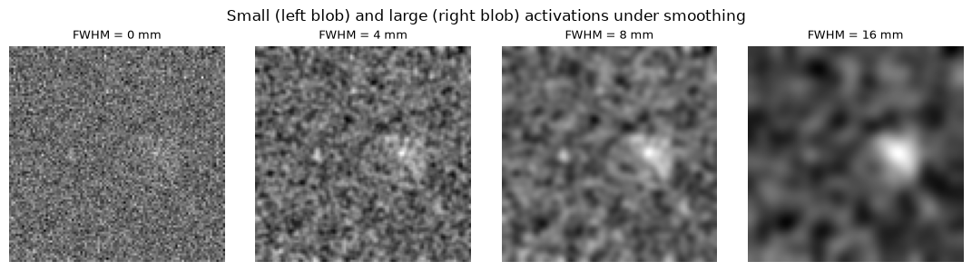
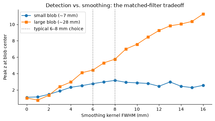
Interpretation. Each activation is best detected with a kernel near its own spatial scale: the small blob’s detectability peaks at a small FWHM and then declines as smoothing dilutes it, while the large blob keeps gaining from heavier smoothing. A single a-priori kernel (the typical 6 or 8 mm) is a compromise — good for cortical-scale signals, costly for fine structure like the brainstem. This is also why MVPA studies analyzing fine-grained patterns often skip smoothing, and why smoothing also serves a second purpose the simulation doesn’t show: making images smooth enough for Gaussian random field theory to yield accurate corrected P values.
Lab 4 — High-pass filter design and drift removal
Scanner drift concentrates power at very low frequencies. High-pass filtering removes it — most transparently by building a set of low-frequency discrete-cosine (DCT) regressors up to the cutoff frequency and projecting them out with the residual-forming matrix
S — residual-forming (filtering) matrix · I — identity matrix · K_H — low-frequency DCT basis (time × regressors) · K_H⁺ — its pseudoinverse
where is the residual-forming matrix that applies the filter, the identity matrix, the matrix of low-frequency DCT regressors (time × regressors), and its Moore–Penrose pseudoinverse.
This is exactly how SPM’s 128-s default works, and it means filtering is nuisance regression. A key practical principle (from the CANlab example linear_filtering_a_timeseries.m, github.com/canlab): do not sequentially filter and then regress out nuisance covariates — combine the DCT columns, motion parameters, spikes, and run intercepts into one matrix and remove them in a single step, and apply the same operation to your task regressors.
# Code adapted from CANlab_help_examples: linear_filtering_a_timeseries.m
TR, n, hpf = 2.0, 300, 128.0   # TR (s); n = volumes; hpf = high-pass cutoff (s)

def dct_highpass_basis(n, TR, cutoff_s):
    """SPM-style DCT basis: cosines with periods longer than the cutoff."""
    k = int(np.floor(2 * n * TR / cutoff_s + 1))
    t = np.arange(n)
    return np.column_stack(
        [np.sqrt(2 / n) * np.cos(np.pi * (2 * t + 1) * j / (2 * n))
         for j in range(1, k)])

KH = dct_highpass_basis(n, TR, hpf)
S = np.eye(n) - KH @ pinv(KH)                   # residual-forming matrix
print(f"{KH.shape[1]} DCT regressors span frequencies below 1/{hpf:.0f} Hz"
      f" = {1/hpf:.4f} Hz")

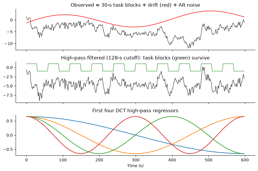
# Simulated run: 30-s alternating blocks + slow drift + AR(2) noise
task = np.tile(np.r_[np.ones(15), np.zeros(15)], 10).astype(float)   # in TRs
tsec = np.arange(n) * TR
drift = 3 * np.sin(2 * np.pi * tsec / 400) + 0.004 * (tsec - tsec.mean())
ar_noise = signal.lfilter([1.0], [1.0, -0.7, -0.3], rng.standard_normal(n))
y_obs = task + drift + ar_noise

y_filt = S @ y_obs
print(f"corr(task, observed) = {np.corrcoef(task, y_obs)[0, 1]:.2f}")
print(f"corr(task, filtered) = {np.corrcoef(task, y_filt)[0, 1]:.2f}")
9 DCT regressors span frequencies below 1/128 Hz = 0.0078 Hz
corr(task, observed) = 0.18
corr(task, filtered) = 0.32
fig, axes = plt.subplots(3, 1, figsize=(9, 6), sharex=True)
axes[0].plot(tsec, y_obs, "k", lw=0.8); axes[0].plot(tsec, drift, "r", lw=1.2)
axes[0].set_title("Observed = 30-s task blocks + drift (red) + AR noise")
axes[1].plot(tsec, y_filt, "k", lw=0.8)
axes[1].plot(tsec, 2 * (task - task.mean()), "g", lw=1.2, alpha=0.7)
axes[1].set_title("High-pass filtered (128-s cutoff): task blocks (green) survive")
axes[2].plot(tsec, KH[:, :4] * 8)
axes[2].set_title("First four DCT high-pass regressors")
axes[2].set_xlabel("Time (s)")
plt.tight_layout()
When the filter eats your task. The filter removes everything below the cutoff — including task signal, if your design puts power there. We measure the fraction of task variance removed, (where is the residual-forming matrix above and the mean-centered task regressor), for alternating block designs of increasing length under the 128-s default.
block_lengths = np.arange(10, 92, 2)            # seconds per block
frac_removed = []
for bl in block_lengths:
    bl_tr = int(round(bl / TR))
    cycles = int(np.ceil(n / (2 * bl_tr)))
    x = np.tile(np.r_[np.ones(bl_tr), np.zeros(bl_tr)], cycles)[:n].astype(float)
    xc = x - x.mean()
    frac_removed.append(1 - (S @ x).var() / xc.var())
frac_removed = np.array(frac_removed)

fig, ax = plt.subplots(figsize=(7, 4))
ax.plot(block_lengths, 100 * frac_removed, "o-")
ax.axvline(64, color="r", ls="--",
           label="64-s blocks: period = 128 s = the cutoff")
ax.set_xlabel("Block length (s), alternating design")
ax.set_ylabel("% of task variance removed by 128-s filter")
ax.legend(); ax.set_title("A default filter can silently delete your effect")
plt.tight_layout()

i32 = np.argmin(np.abs(block_lengths - 32)); i64 = np.argmin(np.abs(block_lengths - 64))
print(f"32-s blocks: {100*frac_removed[i32]:.0f}% of task variance removed")
print(f"64-s blocks: {100*frac_removed[i64]:.0f}% of task variance removed")
32-s blocks: 2% of task variance removed
64-s blocks: 43% of task variance removed
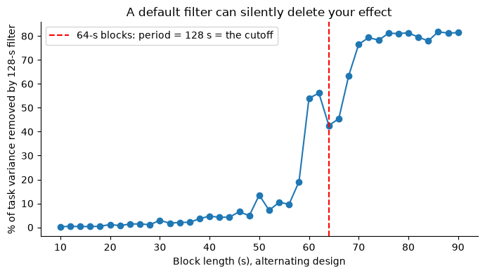
Interpretation. Short alternating blocks sail through the filter, but as the design period approaches the 128-s cutoff the filter removes most of the task variance — with 64-s blocks (128-s period), the “correction” deletes the experiment. This matches the chapter’s warning that default settings can filter out nearly all true signal from designs with alternating blocks of roughly 32 s or longer (where harmonically related power begins to overlap the stopband and losses grow steeply with block length). Always check the overlap between your design’s frequencies and your filter before analyzing — and remember that whatever filter you apply to the data must also be applied to the task regressors and nuisance covariates in your model.
Wrap-up
Realignment parameters capture head motion and explain real variance in voxel time series; FWD summarizes them for censoring, and spike regression censors without destroying temporal structure.
Slice-timing offsets shift sampled responses by up to nearly one TR; interpolation (or regressor-shifting) realigns them in time.
Smoothing is a matched filter: the best kernel depends on the (unknown) signal extent, so the conventional 6–8 mm is a compromise.
High-pass filtering is nuisance regression with DCT cosines; design your cutoff around your task frequencies, not the other way around.
Continue to Chapter 18, where these cleaned-up time series meet the General Linear Model.