Neuroimaging Meta-Analysis
Run this code: ⚡ In-browser lab · Colab · MATLAB Online
Overview
Thousands of neuroimaging papers are now published every year, and at the same time there is growing recognition that results from many small-scale studies are unreliable. False positive rates in neuroimaging are likely higher than in many other fields — a compounding of small samples, massive numbers of tests, analytical variability, and (historically) improper corrections for multiple comparisons; earlier work estimated them at somewhere between 10–40%. Meta-analysis is the primary tool for integrating this literature: it identifies findings that are consistent across labs, scanners, and task variants, and it evaluates how much results vary between studies and why. Across the sciences, cumulative reviews of evidence — assessing overall effect size and generalizability — are often a more useful path to reliable knowledge than a focus on replicating individual studies, and in neuroimaging, meta-analysis is the gold standard way to do this.
Meta-analysis serves three linked goals. Consistency: which regions are reliably activated by a given task or state across the literature, providing a consensus estimate of true activations. Specificity: whether a region’s activation is selective for one psychological process or common to many. A region consistently activated by monetary reward does not license the “reverse inference” that activity there implies reward — that inference is warranted only if the region is not also activated by punishment, memory retrieval, movement planning, and so on. Because individual studies rarely span many psychological domains, meta-analysis provides a unique way to compare activation patterns across the full range of tasks in the literature. Generalizability: whether a region that responds to, say, monetary reward also responds to social and vicarious reward — a window into whether our psychological constructs are biologically coherent categories, and into whether findings replicate across scanners, analysis software, and other methodological choices that ought to be ignorable. Meta-analysis can also map co-activation — regions that tend to be reported together across studies — a meta-analytic analogue of functional connectivity (Chapter 30).
In an ideal world, meta-analysis would pool full statistical maps from every study, fitting a mixed-effects model to effect sizes at each voxel. In practice, full image data are rarely available: individual studies use very different analyses and typically report effect sizes only for a small set of peak activation locations (coordinates in MNI or Talairach space) in published tables. These peak coordinates are the data for coordinate-based meta-analysis (CBMA), either extracted manually from papers or harvested at scale by databases such as Neurosynth, NeuroQuery, and BrainMap. Figure 25.1 shows an example: peak coordinates from 163 studies of emotion, and the map of consistently activated regions estimated from them.
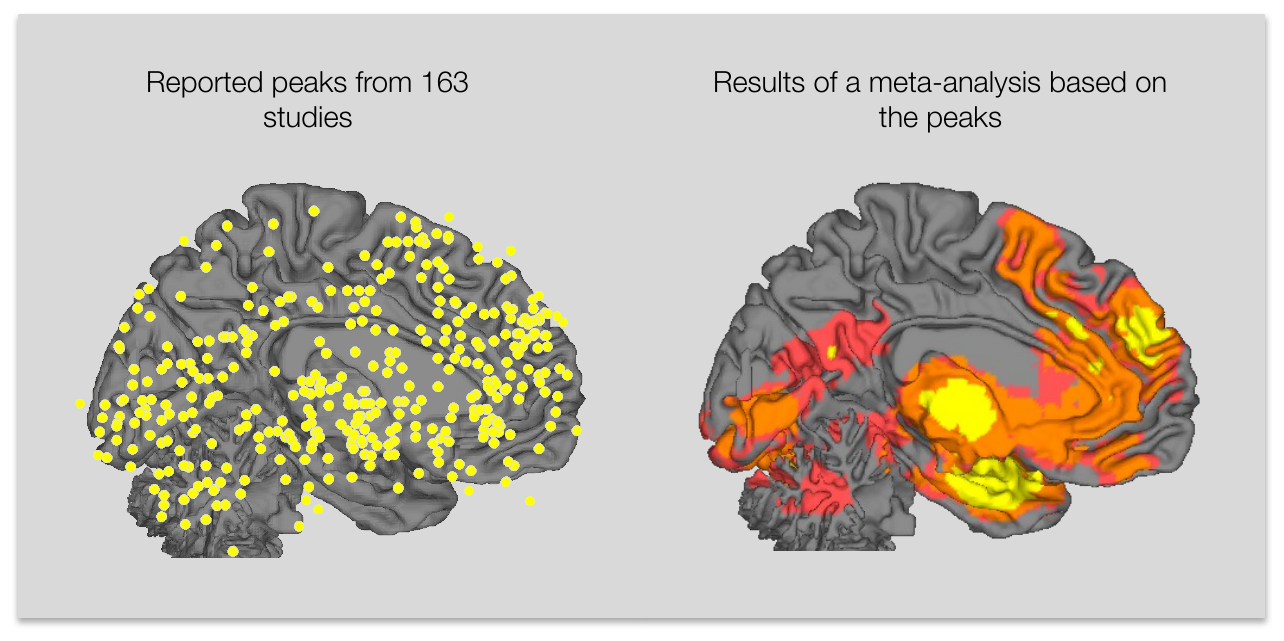
A meta-analysis of emotion. (Left) Peak activation coordinates from 163 studies of emotion. (Right) A summary of consistently activated regions computed using MKDA analysis with the peak coordinates on the left as input. (Figure 25.1 from the book. © the authors and MIT Press; reproduced with permission — not covered by this site’s CC-BY license.)
When effect sizes are available, the classical meta-analytic machinery applies. Each study contributes an effect estimate with sampling variance . A fixed-effects analysis assumes one common true effect and weights each study by its precision, :
θ̂_FE — fixed-effects pooled effect · y_i — effect size from study i · w_i = 1/v_i — precision weight · v_i — sampling variance of study i
where is the fixed-effects pooled effect estimate, the observed effect size from study , its sampling variance, and its precision weight.
A random-effects analysis instead assumes true effects vary across studies with between-study variance , and uses weights . Heterogeneity is quantified with Cochran’s and summarized by , the proportion of total variation attributable to between-study differences. The distinction matters enormously: fixed-effects conclusions apply only to the studies in hand, while random-effects conclusions generalize to the population of studies — and only random-effects models keep a single large (or peak-rich) study from dominating. Publication bias — significant results being more likely to be published — is diagnosed with funnel plots (effect size against precision), where selective publication of significant small-sample results produces a telltale asymmetry and inflates pooled estimates.
The most popular CBMA approaches are kernel-based methods: kernel density approximation (KDA) and activation likelihood estimation (ALE). Both add up peak activations at each voxel and smooth the result with a kernel — spherical with radius in KDA, so the map reads as the number of peaks within mm; Gaussian in ALE, where smoothed values are treated as spatial probability distributions and combined by union into an “activation likelihood.” To threshold the map, Monte Carlo methods simulate the null hypothesis that the reported peaks are uniformly distributed throughout gray matter: random peak sets are generated and smoothed repeatedly, yielding voxel-wise null distributions. KDA saves the maximum density over the brain from each iteration, giving strong family-wise error rate (FWER) control; ALE has typically used false discovery rate (FDR) correction (Chapter 22).
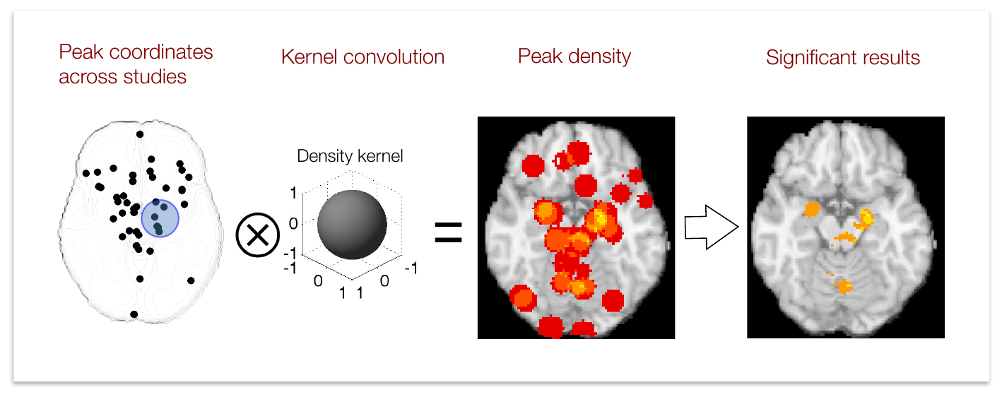
Example of meta-analysis using KDA. Peaks are combined across studies and the resulting map is smoothed with a spherical kernel. The resulting peak density map is thresholded, yielding a map of significant results. (Figure 25.2 from the book. © the authors and MIT Press; reproduced with permission — not covered by this site’s CC-BY license.)
Original KDA and ALE share a critical flaw: the peak is the unit of analysis, so they summarize consistency across peaks rather than across studies. A significant result may be driven entirely by a single study that reports many peaks, and inter-study variability is not modeled at all — the meta-analytic equivalent of a fixed-effects analysis (Chapter 21), and the reason these original versions should not be used. MKDA (multilevel kernel density analysis) and modALE fix this by nesting peaks within study-level contrast maps. In MKDA, each study’s peaks are convolved with a spherical kernel within that study’s map, producing a binary indicator (1 = a peak within mm of this voxel). These indicator maps are then weighted — by sample size () and study quality, downweighting fixed-effects studies — and averaged, so each voxel’s statistic is the weighted proportion of studies activating near it. No single peak-rich study can dominate, and the results generalize beyond the studies analyzed. The Monte Carlo null is refined too: instead of scattering independent peaks, MKDA holds each study’s contiguous activation “blobs” intact and randomizes their locations within gray matter, preserving within-study spatial clustering, with the maximum statistic across iterations providing FWER control. Comparisons between task types use the same machinery on difference maps, and absolute activation differences can be tested with a nonparametric chi-square test on the study-level maps.
User-friendly software makes all of this accessible: GingerALE (BrainMap) for ALE analyses; Neurosynth, which text-mines coordinates from ~14,000 studies and serves forward-inference maps () and reverse-inference maps () online; and the CANlab MKDA toolbox for MATLAB (canlab.github.io). Looking forward, meta-analysis is powering brain-based psychological ontologies, meta-analytic classifiers that predict psychological states from activation, Bayesian spatial models, and priors for multivariate pattern analysis.
Hands-on tutorial
Real coordinate-based meta-analysis needs a curated study database, but every core idea can be seen clearly in simulation — where we know the true effect and can watch pooling, heterogeneity, publication bias, and kernel density estimation do their work. Here are two key steps; the full labs build the complete arc, from simulating a literature through an FWER-thresholded MKDA-style map.
Step 1 — Fixed- vs random-effects pooling. We simulate a literature of studies whose true effects vary around (between-study SD ), then pool with both models. The DerSimonian–Laird estimate of comes straight from Cochran’s .
rng(7);                                  % fix random seed for reproducibility
k     = 25;                              % k = number of studies in the literature
n     = randi([10 80], k, 1);            % per-study sample sizes
theta = 0.3 + 0.2 * randn(k, 1);         % true study effects (tau = 0.2)
d     = theta + randn(k, 1) ./ sqrt(n);  % observed effect sizes
v     = 1 ./ n;                          % sampling variances

w_fe  = 1 ./ v;                          % fixed-effects weights
fe    = sum(w_fe .* d) / sum(w_fe);

Q     = sum(w_fe .* (d - fe).^2);        % Cochran's Q (heterogeneity)
c     = sum(w_fe) - sum(w_fe.^2) / sum(w_fe);
tau2  = max(0, (Q - (k - 1)) / c);       % DerSimonian-Laird tau^2
w_re  = 1 ./ (v + tau2);                 % random-effects weights
re    = sum(w_re .* d) / sum(w_re);

I2    = max(0, (Q - (k - 1)) / Q);       % proportion between-study variation
fprintf('FE = %.3f  RE = %.3f  tau2 = %.3f  I2 = %.0f%%\n', fe, re, tau2, 100 * I2);
import numpy as np
rng = np.random.default_rng(7) # fix random seed for reproducibility
k = 25 # k = number of studies in the literature
n = rng.integers(10, 81, k) # per-study sample sizes
theta = 0.3 + 0.2 * rng.standard_normal(k) # true study effects (tau = 0.2)
d = theta + rng.standard_normal(k) / np.sqrt(n) # observed effect sizes
v = 1 / n # sampling variances
w_fe = 1 / v # fixed-effects weights
fe = np.sum(w_fe * d) / np.sum(w_fe)
Q = np.sum(w_fe * (d - fe) ** 2) # Cochran's Q (heterogeneity)
c = np.sum(w_fe) - np.sum(w_fe ** 2) / np.sum(w_fe)
tau2 = max(0, (Q - (k - 1)) / c) # DerSimonian-Laird tau^2
w_re = 1 / (v + tau2) # random-effects weights
re = np.sum(w_re * d) / np.sum(w_re)
I2 = max(0, (Q - (k - 1)) / Q) # proportion between-study variation
print(f"FE = {fe:.3f} RE = {re:.3f} tau2 = {tau2:.3f} I2 = {100 * I2:.0f}%")Example output:
FE = 0.218 RE = 0.208 tau2 = 0.024 I2 = 53%With , over half the variation between studies reflects genuine differences in true effects — and the random-effects estimate accordingly differs from (and generalizes beyond) the fixed-effects one.
Step 2 — An MKDA-style density map from peak coordinates. Working on a 2D “axial slice” for speed, each study’s peaks become a binary indicator map (1 within mm of any peak), and the MKDA statistic is the weighted proportion of study maps active at each location. The full labs contrast this with peak-level KDA — showing how one peak-rich study can hijack a fixed-effects map — and add the Monte Carlo max-statistic threshold.
% peaks_by_study: {k x 1} cell, each an [n_peaks x 2] matrix of x,y (mm)
% n:              [k x 1] sample sizes, one per study
% Adapted from CANlab MKDA tools logic (github.com/canlab/Canlab_MKDA_MetaAnalysis)
r = 10;                                        % kernel radius (mm)
[xx, yy] = meshgrid(-90:2:90, -126:2:90);      % 2 mm grid, MNI-like slice
grid_xy = [xx(:) yy(:)];

k = numel(peaks_by_study);                     % k = number of studies
maps = zeros(k, size(grid_xy, 1));             % one indicator map per study
for i = 1:k
    pk = peaks_by_study{i};                    % squared distance to each peak
    d2 = (grid_xy(:, 1) - pk(:, 1)').^2 + (grid_xy(:, 2) - pk(:, 2)').^2;
    maps(i, :) = min(d2, [], 2) <= r^2;        % 1 if within r mm of any peak
end

w = sqrt(n); w = w / sum(w);                   % sqrt(N) study weights
mkda = w' * maps;                              % weighted proportion of studies
mkda_map = reshape(mkda, size(xx));
imagesc([-90 90], [-126 90], mkda_map); axis image; colorbar;
In a real analysis with the CANlab MKDA toolbox, the same logic runs in 3D on a coordinate database, with FWER thresholding, in two lines:
DB = Meta_Setup(DB, 10);                             % 10 mm kernel, sqrt(N) weights
Meta_Activation_FWE('all', DB, 5000, 'nocontrasts'); % maps + Monte Carlo + results
import matplotlib.pyplot as plt
# peaks_by_study: list of k arrays, each (n_peaks, 2) of x, y coordinates (mm)
# n: array of k sample sizes, one per study
r = 10 # kernel radius (mm)
xx, yy = np.meshgrid(np.arange(-90, 91, 2), # 2 mm grid, MNI-like slice
np.arange(-126, 91, 2))
grid_xy = np.column_stack([xx.ravel(), yy.ravel()])
def study_indicator(peaks):
"""Binary map: 1 within r mm of any of this study's peaks."""
d2 = ((grid_xy[:, None, :] - peaks[None, :, :]) ** 2).sum(axis=-1)
return (d2.min(axis=1) <= r ** 2).astype(float)
maps = np.array([study_indicator(p) for p in peaks_by_study]) # one map per study
w = np.sqrt(n); w = w / w.sum() # sqrt(N) study weights
mkda = w @ maps # weighted proportion of studies
mkda_map = mkda.reshape(xx.shape)
plt.imshow(mkda_map, origin="lower", extent=[-90, 90, -126, 90]); plt.colorbar()Example output:
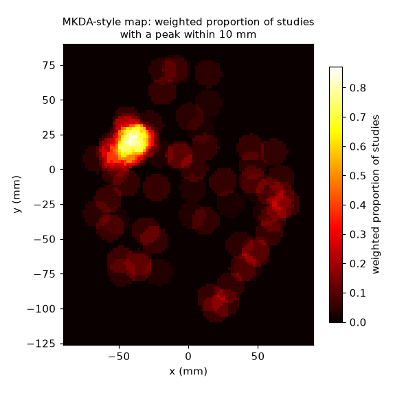
With 20 simulated studies, the weighted proportion of studies with a peak within 10 mm reaches 0.87 at the true region near mm, while isolated single-study peaks appear only faintly — the consistency signal meta-analysis is designed to isolate.
Open the full Python lab notebook → or download the MATLAB live script, which mirrors it and points to the CANlab MKDA toolbox for real 3D analyses. Both labs simulate a literature with a publication filter, compare fixed- and random-effects pooling with forest plots, diagnose bias with funnel plots, and build an FWER-thresholded MKDA-style map.


Thought questions
A colleague sees amygdala activation in their study and concludes participants were experiencing fear. Using the concepts of consistency and specificity, explain what meta-analytic evidence would be needed to justify (or undermine) this reverse inference, and why no single study can provide it.
Coordinate-based meta-analysis inherits a subtle form of publication bias even before whole studies go missing: tables report only peaks that survived each study’s threshold. How does this within-study selection distort a KDA/ALE/MKDA map, and how would its effects differ from classic “file-drawer” publication bias in an effect-size meta-analysis?
Suppose your MKDA analysis of “cognitive control” yields a significant anterior cingulate cluster, but you discover that in the corresponding effect-size data is very high. What sources of heterogeneity — psychological, methodological, and statistical — would you investigate, and how could meta-analysis itself help decide whether “cognitive control” is a coherent construct?
The original KDA and ALE methods are described as performing “the equivalent of a fixed-effects analysis.” Trace exactly how a single study reporting 40 peaks could produce a significant cluster in KDA, and explain — mechanistically — how MKDA’s design (indicator maps, weighting, blob-level randomization) prevents each part of the problem.
If all future studies deposited full statistical maps in public repositories, which parts of the meta-analytic toolkit described in this chapter would become obsolete, which would remain essential, and what new problems (e.g., analytical variability across pipelines) would move to center stage?
Quiz yourself
Q1. What three properties of neuroimaging findings does meta-analysis help establish?
Answer: Consistency (which regions are reliably activated across studies), specificity (whether activation is selective for one psychological process or shared by many), and generalizability (whether effects hold across task subtypes, scanners, and methodological choices).
Q2. Why is most neuroimaging meta-analysis coordinate-based rather than based on full statistical maps?
Answer: Full image data are rarely shared, and individual studies use very different analyses. What is consistently available are the peak activation coordinates (in MNI or Talairach space) reported in published tables, so these coordinates become the data for meta-analysis.
Q3. What is the difference between fixed-effects and random-effects pooling, and which supports generalization beyond the studies analyzed?
Answer: Fixed-effects analysis assumes a single common true effect and weights studies by ; random-effects analysis assumes true effects vary across studies with variance and weights by . Only random-effects conclusions generalize to the broader population of studies.
Q4. What do Cochran’s , , and measure?
Answer: All three quantify heterogeneity. is the weighted sum of squared deviations of study effects from the fixed-effects pooled estimate; estimates the variance of true effects between studies; and expresses the proportion of total variation in observed effects attributable to between-study differences rather than sampling error.
Q5. How do the kernels differ between KDA and ALE, and how is each map interpreted?
Answer: KDA convolves peaks with a spherical kernel of radius , so the map counts peaks within mm of each voxel. ALE uses a Gaussian kernel, treats the smoothed values as spatial probability distributions, and computes their union — interpreted as the probability that at least one peak lies at that voxel.
Q6. What null hypothesis do the Monte Carlo procedures simulate, and how does KDA achieve family-wise error control?
Answer: The null hypothesis is that the reported peaks are uniformly distributed throughout gray matter. Random peak sets are generated and smoothed repeatedly; KDA saves the maximum density value from each iteration, building a max-statistic distribution whose quantiles give thresholds with strong FWER control.
Q7. Why should the original KDA and ALE not be used, and what two key changes do MKDA and modALE introduce?
Answer: The originals treat peaks as the unit of analysis, so a single study reporting many peaks can drive significance, and inter-study variability is unmodeled — a fixed-effects analysis. MKDA/modALE nest peaks within study-level contrast maps (the study becomes the unit, treated as a random effect) and weight maps by sample size and study quality, so results generalize and no single study dominates.
Q8. In a funnel plot, what pattern suggests publication bias, and what is the consequence for the pooled effect?
Answer: Publication bias produces asymmetry: small, imprecise studies appear only when their effects are large enough to be significant, so the lower part of the funnel is missing on the null side. The surviving studies overestimate the effect, inflating the pooled estimate.
 The book: Elements of Functional Magnetic Resonance Imaging — Wager & Lindquist, MIT Press