Image Preprocessing
Run this code: ⚡ In-browser lab · Colab · MATLAB Online
Overview
Before any statistical analysis, fMRI data pass through a sequence of preprocessing steps with three aims: (1) minimize the influence of artifacts from data acquisition and head movement; (2) transform the data so it better meets statistical assumptions; and (3) for group analysis, standardize the locations of brain regions across individuals. The typical pipeline — reconstruction, distortion correction, slice-timing correction, motion correction (realignment), coregistration of structural and functional images, spatial normalization, smoothing, temporal filtering, and physiological noise correction — is summarized below. A recurring theme runs through every step: each correction removes a mixture of artifact and real signal, so each involves a tradeoff that is worth understanding rather than accepting on faith.
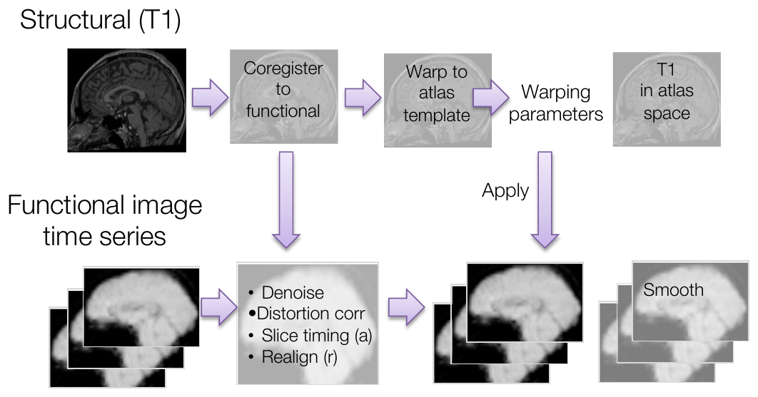
An example preprocessing pipeline. The structural (T1) image is coregistered to the functional images and warped to an atlas template; the resulting warping parameters are then applied to the functional time series, which has itself been denoised, distortion-corrected, slice-time corrected, and realigned. Smoothing comes last. (Figure 17.1 from the book. © the authors and MIT Press; reproduced with permission — not covered by this site’s CC-BY license.)
Reconstruction and artifact checks. Images are acquired in k-space and reconstructed into image space at the scanner, stacked into 3-D volumes (one per TR), and aggregated into 4-D NIfTI files whose headers record voxel size, TR, TE, and more. This is the moment to check for scanner artifacts and distortions — sometimes with surprising results: one early PET study localized “anticipatory pain activation” to the temporal pole, which turned out to be the jaw of subjects clenching their teeth.
EPI distortion correction. Susceptibility artifacts cause signal loss and geometric warping of functional EPI images, especially near air–tissue boundaries (orbitofrontal cortex, temporal poles, brainstem), producing nonlinear mismatches with the anatomical image. Two main corrections exist, both based on extra scans acquired before the functional runs. Unwarping collects a B0 field map, estimates voxel displacement from field inhomogeneity, and applies the inverse. Reverse-blip methods acquire brief EPI scans with opposite phase-encoding directions (A–P and P–A); distortion is maximal along the phase-encoding axis with opposite sign in the two scans, so algorithms such as FSL’s topup interpolate to the midpoint. Distortion correction is recommended — without it, functional images do not align well with structural images or atlases — but it is not magic: correction can over-correct, introducing new artifacts.
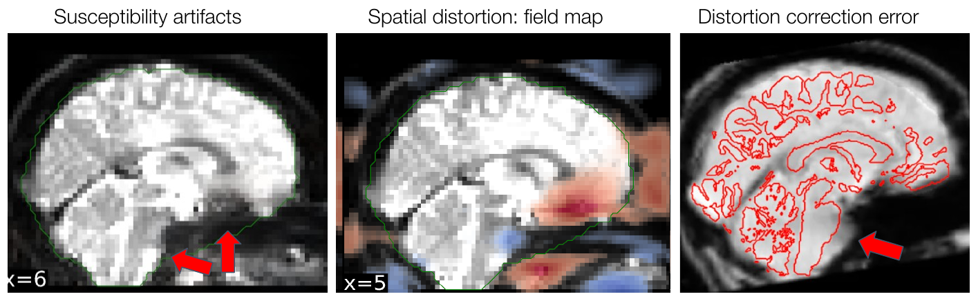
Distortion correction. Left: a functional EPI image with characteristic distortion in orbitofrontal cortex and brainstem. Center: estimated distortion along the phase-encoding direction from a reverse-blip acquisition (red = expansion, blue = compression). Right: correction improves the match to the T1 anatomy but can also over-correct — here functional signal is expanded beyond the brainstem boundary. (Figure 17.2 from the book. © the authors and MIT Press; reproduced with permission — not covered by this site’s CC-BY license.)
Slice-timing correction. Slices within a volume are acquired at different times, but analyses treat each volume as a snapshot. Slice-timing correction interpolates each voxel’s time series to the acquisition time of a reference slice (often the middle of the TR). Getting the actual acquisition order right — sequential vs. interleaved — is essential; assuming the wrong order does harm. Interpolation always introduces some error, can interact badly with head motion, and can smear transient “spike” artifacts in time. With modern rapid acquisitions (TR ≤ 1 s), it is increasingly common to skip slice-timing correction entirely and instead shift the task regressors per slice or use flexible hemodynamic basis sets. Correction matters more as TR grows, for brief events, and for resting-state connectivity at long TRs, where timing offsets between regions distort correlations.
Motion correction (realignment). Head motion is among the most serious artifact sources in fMRI: a voxel’s time series is only meaningful if it samples the same brain location at every time point. Realignment registers each volume to a reference (the first or mean image) using a rigid-body transformation with 6 parameters — translations in and rotations (roll, pitch, yaw) — estimated by iteratively minimizing squared differences between images. The six parameter time courses are saved and routinely used as nuisance covariates in the GLM. Realignment does not fix everything: spin-history effects persist during and after movement. Additional defenses include head restraints and participant training, prospective motion correction, motion covariates in the GLM, and censoring high-motion volumes. Censoring uses framewise displacement, the sum of absolute frame-to-frame changes in the six parameters, with rotations converted to millimeters as arc length on a sphere of radius 50 mm (roughly the cortex-to-center distance):
FWDₜ — framewise displacement at frame t (mm) · Δd — frame-to-frame change in each translation (mm) · Δα, Δβ, Δγ — changes in the three rotations (radians) · 50 — sphere radius (mm) converting rotation to arc length
where is the framewise displacement at frame , are the frame-to-frame changes in the three translations (in mm), the changes in the three rotations (in radians), and the factor 50 converts rotations to millimeters of arc length on a 50-mm-radius sphere.
Volumes exceeding a threshold (0.2–0.5 mm is typical for resting state) are removed by “scrubbing” or — preferably — modeled with spike regression, one nuisance regressor per bad image, which preserves the natural temporal correlation structure for inference. Typical mean FWD is about 0.05 mm in healthy young adults, 0.10 mm in the population-based UK Biobank, and 0.2–0.4 mm in children; a mean-FWD cutoff around 0.25 mm excludes only the worst runs in adults. But beware selection bias: motion is heritable, correlated with body-mass index and clinical variables, and can correlate with task states — so aggressive exclusion of images, runs, or participants can mask true effects or manufacture spurious ones. Conservative censoring plus vigorous motion prevention (padding, tape for tactile feedback, coaching, mock-scanner training) is the recommended combination.
Coregistration. The session’s high-resolution structural image must be aligned to the functional images, both for visualization and so that normalization estimated from the detailed T1 can be applied to the functionals. A rigid-body transform is used, but minimizing squared intensity differences is inappropriate across modalities — tissue intensities are ordered W > G > V in functional images and V > G > W in structural images — so coregistration instead maximizes mutual information. Coregistration is a common failure point, largely because susceptibility distortions differ across modalities; checking it for every participant is essential quality control.
Normalization. Group analysis requires each voxel to correspond to the same brain region in every subject. Normalization registers each subject’s anatomy to a standardized atlas space defined by a template — usually a group-average brain in volume or surface space. Linear (affine) registration adds scaling and shearing to the rigid-body parameters but is too coarse on its own; nonlinear algorithms (SPM’s unified segmentation, FSL’s FNIRT, ANTs) use smooth 3-D basis functions to locally stretch and shrink the image. Surface-based normalization (FreeSurfer) instead treats the cortex as a sheet and aligns folding patterns — consistently outperforming volumetric methods for cortex, and enabling smoothing that does not mix signals across gyri or into non-gray tissue. Flexibility is a double-edged sword: too many unconstrained basis functions overfit local features and can grossly distort overall brain shape (a “local minimum” solution), while too-rigid warps leave individuals poorly aligned. Inter-subject registration is one of the largest sources of error in group analysis, so inspect every normalized brain.
The choice of template matters more than many realize. “MNI space” is not one thing: MNI305, MNI152, ICBM2009 (symmetric and asymmetric variants), IXI555, and others differ in resolution, sharpness, the locations of some structures, and even the origin, shifting the whole brain relative to other templates. Report the exact template you used, and check that anatomical atlases used for localization match it.
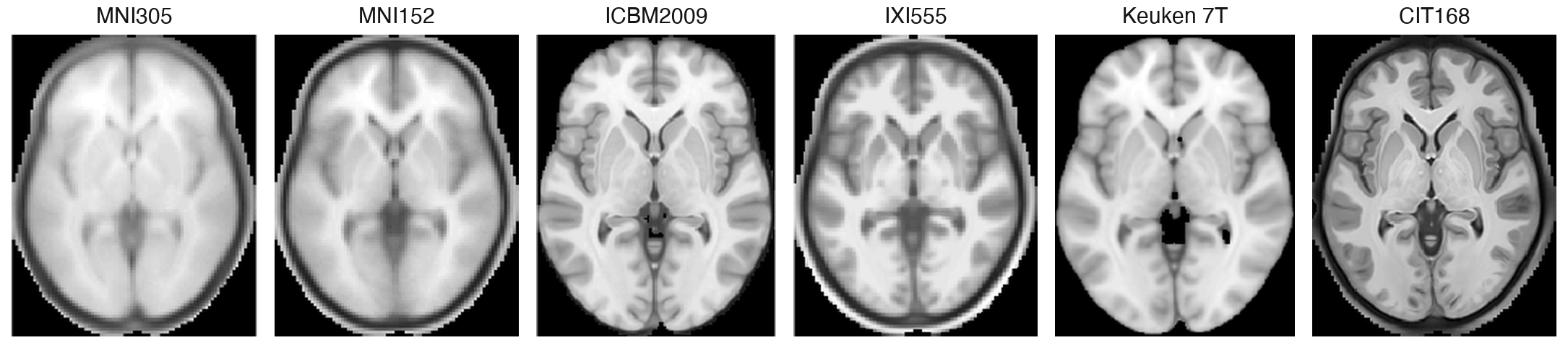
Templates normalized to MNI space are broadly similar but differ in resolution, smoothness, and the locations of some structures. MNI305 and MNI152 were common targets in the 2000s; higher-definition templates such as ICBM2009 and IXI555 have gradually replaced them. (Figure 17.5 from the book. © the authors and MIT Press; reproduced with permission — not covered by this site’s CC-BY license.)
Spatial smoothing. Smoothing convolves the data with a 3-D Gaussian kernel characterized by its full width at half maximum, , where is the standard deviation of the Gaussian kernel in millimeters. It compensates for residual anatomical misalignment after normalization and satisfies the smoothness assumptions of Gaussian random field theory for multiple-comparisons correction. The cost is partial-volume mixing: averaging truly active voxels with null neighbors dilutes signal. In theory, a kernel matched to the spatial extent of the activation is optimal (the matched-filter idea), but in practice one fixed kernel — typically 6 or 8 mm — is applied everywhere, even though signals in cortex are smoother than in the brainstem. MVPA studies often skip smoothing to preserve fine-grained patterns, though modest smoothing can actually help when decoding across participants.
Temporal filtering. Each voxel’s time series contains slow scanner drift and low-frequency noise; high-pass filtering removes it, either by adding low-frequency cosine covariates to the GLM or by premultiplying data and regressors with a filtering matrix (frequency-domain filtering via the Fourier transform is equivalent). The critical rule: your task frequencies must not overlap the filter’s stopband. SPM’s default 128-s (0.0078 Hz) cutoff will remove nearly all true signal from designs with alternating blocks of about 32 s or longer — producing null results no matter how strong the effect. Resting-state analyses typically band-pass at 0.01–0.08 Hz, which brackets the canonical HRF’s peak frequency (~0.03 Hz) and excludes much respiratory (0.08–0.4 Hz) and aliased cardiac noise, though interest in faster BOLD components is growing. Physiological noise correction (e.g., RETROICOR, RVHRCOR) uses recorded respiration and pulse to build nuisance regressors — with the same caveat that closes the loop on this chapter’s theme: tasks change physiology, so corrections remove real signal along with artifact, and they help only when the artifact removed outweighs the signal lost.
Hands-on tutorial
Real preprocessing runs inside packages like SPM, FSL, and fMRIPrep — but every step is easier to reason about once you have simulated it yourself. Here we look at two steps you can fully understand in a few lines of code: using realignment parameters as nuisance regressors, and designing a high-pass filter that removes drift without removing your task. The full labs add slice-timing and smoothing-kernel simulations.
Step 1 — Motion parameters as nuisance regressors. We simulate a voxel time series contaminated by head motion, then quantify how much variance the six realignment parameters explain.
% Requires CanlabCore + SPM12 on your MATLAB path
% Adapted from CANlab tutorials (github.com/canlab)
rng(17);           % seed the random-number generator for reproducibility
n = 200; TR = 1;   % n = volumes (frames); TR = repetition time (s)

% 6 motion params (random walk): 3 translations (mm), 3 rotations (radians)
mp = cumsum(0.02 * randn(n, 6));
mp(:, 4:6) = mp(:, 4:6) * 0.005;              % rotations are small in radians
mp(120:124, 1:3) = mp(120:124, 1:3) + 0.8;    % a sudden 0.8 mm head jerk
mp(120:124, 4:6) = mp(120:124, 4:6) + 0.004;  % with a small rotation component

true_signal = noise_arp(n, [.5 .1]);   % "neural" fluctuations, AR(2)
w = [2 1.5 1 300 200 100]';            % motion-artifact coupling weights
y = true_signal + mp * w + 0.5 * randn(n, 1);   % voxel = signal + artifact + noise

% Variance explained by motion parameters (R^2 from nuisance regression)
X  = [mp ones(n, 1)];      % design: 6 motion params + intercept
r  = y - X * (X \ y);      % residuals after regressing out motion
R2 = 1 - var(r) / var(y);
fprintf('Motion explains %.0f%% of voxel variance\n', 100 * R2)

% Framewise displacement: |diffs| summed, rotations (radians) x 50 mm
fwd = sum(abs(diff(mp(:, 1:3))), 2) + 50 * sum(abs(diff(mp(:, 4:6))), 2);
thresh = 0.5;              % censoring threshold (mm); 0.2-0.5 mm is typical
fprintf('%d frames exceed a %.1f mm censoring threshold\n', sum(fwd > thresh), thresh)
create_figure('FWD'); plot([0; fwd]); plot_horizontal_line(thresh);
xlabel('Frame'); ylabel('FWD (mm)');
import numpy as np
import matplotlib.pyplot as plt
rng = np.random.default_rng(17) # seed for reproducibility
n, TR = 200, 1.0 # n = volumes (frames); TR = repetition time (s)
# 6 motion params (random walk): 3 translations (mm), 3 rotations (radians)
mp = np.cumsum(0.02 * rng.standard_normal((n, 6)), axis=0)
mp[:, 3:] *= 0.005 # rotations are small in radians
mp[120:125, :3] += 0.8 # a sudden 0.8 mm head jerk at frame 120
mp[120:125, 3:] += 0.004 # with a small rotation component
# AR(2)-like "neural" fluctuations plus motion-coupled artifact
true_signal = np.convolve(rng.standard_normal(n), [1, .5, .1])[:n]
w = np.array([2, 1.5, 1, 300, 200, 100]) # motion-artifact coupling weights
y = true_signal + mp @ w + 0.5 * rng.standard_normal(n)
# Variance explained by motion parameters (R^2 from nuisance regression)
X = np.column_stack([mp, np.ones(n)]) # design: 6 motion params + intercept
resid = y - X @ np.linalg.lstsq(X, y, rcond=None)[0]
print(f"Motion explains {100 * (1 - resid.var() / y.var()):.0f}% of variance")
# Framewise displacement: |diffs| summed, rotations (radians) x 50 mm
fwd = (np.abs(np.diff(mp[:, :3], axis=0)).sum(1)
+ 50 * np.abs(np.diff(mp[:, 3:], axis=0)).sum(1))
thresh = 0.5 # censoring threshold (mm); 0.2-0.5 mm is typical
print(f"{(fwd > thresh).sum()} frames exceed a {thresh} mm censoring threshold")
fig, ax = plt.subplots(figsize=(7, 3))
ax.plot(np.r_[0, fwd], "k", lw=0.9) # prepend 0: frame 1 has no predecessor
ax.axhline(thresh, color="r", ls="--", label=f"{thresh} mm censoring threshold")
ax.set_xlabel("Frame"); ax.set_ylabel("FWD (mm)")
ax.set_title("Framewise displacement"); ax.legend()Example output:
Motion explains 53% of variance
2 frames exceed a 0.5 mm censoring threshold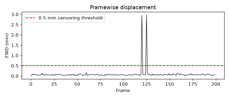
The FWD trace flags exactly the frames where the simulated head jerk begins and ends — these two frames would each get a spike regressor.
Step 2 — High-pass filtering without destroying the task. We build a discrete-cosine high-pass filter (the same construction SPM uses) and apply it as a residual-forming matrix, following the CANlab principle that filtering and nuisance regression should happen in one step.
% Adapted from CANlab_help_examples: linear_filtering_a_timeseries.m
TR = 2; n = 300; hpf = 128;   % TR (s); n = volumes; hpf = high-pass cutoff (s)

[S, KL, KH] = use_spm_filter(TR, n, 'none', 'specify', hpf);
% KH: low-frequency cosine regressors; S: residual-forming matrix

task  = repmat([ones(15, 1); zeros(15, 1)], 10, 1);   % 30-s alternating blocks (15 TRs on, 15 off)
drift = 4 * cos((1:n)' * 2 * pi / 280);               % slow scanner drift (280-s period)
y_obs = task + drift + noise_arp(n, [.7 .3]);

y_filt = S * y_obs;                                % drift removed
fprintf('corr(task, observed) = %.2f, corr(task, filtered) = %.2f\n', ...
    corr(task, y_obs), corr(task, y_filt))

% Danger check: how much TASK variance does the filter remove?
task_lost = 1 - var(S * task) / var(task - mean(task));
fprintf('Filter removes %.0f%% of task variance\n', 100 * task_lost)
import numpy as np
from scipy.linalg import pinv
TR, n, hpf = 2.0, 300, 128.0 # TR (s); n = volumes; hpf = high-pass cutoff (s)
# Discrete-cosine high-pass basis (SPM's construction)
k = int(np.floor(2 * n * TR / hpf + 1)) # of basis functions below the cutoff
t = np.arange(n) # frame indices 0..n-1
KH = np.column_stack([np.sqrt(2 / n) * np.cos(np.pi * (2 * t + 1) * j / (2 * n))
for j in range(1, k)])
S = np.eye(n) - KH @ pinv(KH) # residual-forming matrix
task = np.tile(np.r_[np.ones(15), np.zeros(15)], 10) # 30-s blocks (15 TRs on, 15 off)
drift = 4 * np.cos(np.arange(n) * 2 * np.pi / 280) # slow drift (280-s period)
rng = np.random.default_rng(0) # seed for reproducibility
y_obs = task + drift + rng.standard_normal(n)
y_filt = S @ y_obs # drift removed
print(f"corr(task, observed) = {np.corrcoef(task, y_obs)[0,1]:.2f}, "
f"filtered = {np.corrcoef(task, y_filt)[0,1]:.2f}")
# Danger check: how much TASK variance does the filter remove?
task_c = task - task.mean()
print(f"Filter removes {100 * (1 - (S @ task).var() / task_c.var()):.0f}% "
"of task variance")Example output:
corr(task, observed) = 0.17, filtered = 0.44
Filter removes 3% of task variance
With 30-s alternating blocks (60-s period), the 128-s filter leaves the task nearly untouched while removing the drift. Re-run the same code with 64-s blocks (128-s period) and watch the filter remove most of your task variance — the exact failure mode the chapter warns about. The full labs continue with a slice-timing offset demo and a smoothing-kernel tradeoff simulation.
Open the full Python lab notebook → or download the MATLAB live script, which mirrors it using CANlab tools.


Thought questions
Every preprocessing step removes a mixture of artifact and true signal. Pick two steps (e.g., high-pass filtering and physiological noise correction) and describe a concrete experiment in which each would reduce your power to detect a true effect. What could you change — in the design or the preprocessing — to shift the balance back?
A collaborator proposes excluding all participants with mean FWD above 0.1 mm from a study comparing adolescents with and without ADHD. Drawing on what you know about who moves more and why, explain the selection-bias risks, and propose a defensible alternative motion-handling strategy.
Slice-timing correction and motion correction each involve interpolation, and their errors interact — a voxel that moves samples different brain locations at different times. Discuss the arguments for the order of these two steps, and why rapid multiband acquisition changes the calculus (for both task and resting-state analyses).
Two labs analyze the same dataset. One normalizes volumetrically to MNI152 with aggressive nonlinear warping; the other uses surface-based normalization with modest smoothing on the cortical sheet. For which brain structures and which scientific questions would you expect their results to diverge most, and why?
Your task alternates 45-s blocks of pain and rest, and your software’s default high-pass cutoff is 128 s. Walk through what happens to your task effect, how you would detect the problem from the data and design (not just from a null result), and two distinct ways to fix it.
Quiz yourself
Q1. What are the three broad aims of fMRI preprocessing?
Answer: (1) Minimize the influence of artifacts from acquisition and head movement; (2) check and transform the data to better meet statistical assumptions; and (3) for group analyses, standardize the locations of brain regions across individuals.
Q2. What are the two main approaches to EPI distortion correction, and what extra data does each require?
Answer: Unwarping uses a B0 field map scan to estimate signal displacement from field inhomogeneity and applies the inverse. Reverse-blip methods (e.g., FSL’s topup) acquire brief additional EPI scans with opposite phase-encoding directions (A–P and P–A) and interpolate the images to the midpoint of the two opposite distortions.
Q3. How many parameters does rigid-body realignment estimate, and what are they?
Answer: Six: three translations (shifts along x, y, and z) and three rotations (roll, pitch, and yaw). They are estimated by iteratively minimizing the squared difference between each volume and a reference image, and saved for use as nuisance covariates.
Q4. How is framewise displacement (FWD) computed, and how are rotations handled?
Answer: FWD is the sum of the absolute frame-to-frame changes (temporal derivatives) of the six realignment parameters. Rotations are first converted to millimeters by computing arc length on a sphere of radius 50 mm — approximately the distance from the cortex to the center of the brain.
Q5. Why is minimizing squared intensity differences inappropriate for coregistering structural to functional images, and what is used instead?
Answer: Because tissue classes have different intensity orderings in the two modalities — white > gray > ventricles in functional (T2*) images but ventricles > gray > white in structural (T1) images — the same anatomy does not have matching intensities. Coregistration therefore maximizes mutual information between the images instead.
Q6. Why is spike regression generally preferred over scrubbing for censoring high-motion volumes?
Answer: Spike regression adds one nuisance regressor per bad image within the GLM, which removes the volume’s influence while preserving the natural temporal correlation structure of the time series — important for valid statistical inference (P values). Scrubbing physically deletes volumes, disrupting temporal structure.
Q7. Give two reasons fMRI data are spatially smoothed, and the main cost of smoothing.
Answer: Smoothing blurs residual anatomical misalignment left over from normalization, and it makes images smooth enough for Gaussian random field theory to give accurate corrected P values. The cost is partial-volume mixing: signal from truly active regions is averaged with null neighbors, reducing effective signal and blurring fine spatial patterns (one reason MVPA studies often skip it).
Q8. Your design alternates 40-s task and 40-s rest blocks. What happens if you apply SPM’s default 128-s high-pass filter, and why?
Answer: The task’s fundamental frequency (1/80 s = 0.0125 Hz) is close to the filter’s 0.0078 Hz cutoff, and designs with alternating blocks of roughly 32 s or longer have substantial power at or below the cutoff — so the filter removes much of the true task-related signal, sharply reducing power (potentially to near zero for longer blocks) regardless of the true effect size.
 The book: Elements of Functional Magnetic Resonance Imaging — Wager & Lindquist, MIT Press