Real fMRI noise is not a featureless hiss: it drifts, it repeats itself, it spikes, and it carries the imprint of the beating heart. In this lab you will build an fMRI-like time series from its noise ingredients, then learn to diagnose each one:
Simulate a noisy voxel from known components: slow drift, AR(1) autocorrelated noise, transient spikes, and a heartbeat sampled at the TR
Move to the frequency domain to see 1/f drift and demonstrate temporal aliasing — including why a 1 Hz heartbeat shows up as low-frequency noise
Detect transient outliers in a multi-voxel dataset with RMSSD/DVARS and Mahalanobis distance, and build spike regressors
Measure what autocorrelation does to naive OLS — and fix it with prewhitening
Because we build the noise ourselves, we know the ground truth, so every diagnostic can be checked against what we put in.
How to run this notebook. Run it in your browser from the tutorial site, in Google Colab, or in a local Jupyter installation. It uses only numpy, scipy, pandas, and matplotlib, and all data are simulated — nothing to download. It accompanies the chapter page.
▶ This notebook is interactive. Click the ⏻ power icon at the top right of this page to run it in your browser — no installation needed (the kernel takes ~30–60 s to start the first time). Then run cells top to bottom, starting with the first code cell below: later cells depend on the imports and variables defined earlier, and will error if you skip ahead.
import numpy as np
import pandas as pd
import matplotlib.pyplot as plt
from scipy import stats, signal

rng = np.random.default_rng(7)             # seed for reproducibility
np.set_printoptions(precision=3, suppress=True)   # compact array printing
print("numpy", np.__version__)
numpy 2.4.6
Part 1 — Anatomy of a noisy voxel time series
We simulate an 8-minute run (240 volumes, TR = 2 s) and add up four noise ingredients on top of a constant baseline of 100:
Slow drift — a sum of slow cosines, mimicking scanner instability and slow physiological change. In real data, drift power grows in inverse proportion to frequency (“1/f noise”).
AR(1) autocorrelated noise — noise that “remembers” its recent past:
ε_t — noise value at time t · φ — autoregressive (autocorrelation) coefficient · η_t — new independent Gaussian noise at time t · σ² — variance of the new noise
where is the noise value at time , the autoregressive (autocorrelation) coefficient, the new independent Gaussian noise added at time , and its variance.
With , each time point inherits half of the previous deviation, so errors are correlated across time.
A heartbeat — simulated at high temporal resolution (50 Hz) as a train of pulses at ~60 beats/min with natural beat-to-beat jitter, then sampled once per TR, exactly as the scanner does.
Transient spikes — three volumes with sudden intensity shifts, standing in for gradient glitches or abrupt head movement.
TR, n = 2.0, 240                          # TR = repetition time (s); n = volumes (8-min run)
t = np.arange(n) * TR                     # volume acquisition times (s)

# --- Slow drift: sum of slow cosines -------------------------------------
drift = 6 * np.cos(2 * np.pi * t / 400) + 3 * np.cos(2 * np.pi * t / 180)

# --- AR(1) noise, phi = 0.5 ----------------------------------------------
phi = 0.5                                 # AR(1) coefficient: each error keeps half the last
eta = rng.standard_normal(n)
ar1 = signal.lfilter([1.0], [1.0, -phi], eta)   # e_t = phi*e_{t-1} + eta_t

# --- Heartbeat at ~60 bpm, built at 50 Hz then sampled at the TR ---------
dt = 0.02                                 # high-resolution time step (s)
t_hi = np.arange(0, n * TR, dt)
beats = np.cumsum(rng.normal(1.0, 0.05, size=int(n * TR * 1.3)))  # jittered
beats = beats[beats < t_hi[-1]]
hb_hi = np.zeros_like(t_hi)
for b in beats:                           # each beat: a narrow pulse
    hb_hi += np.exp(-0.5 * ((t_hi - b) / 0.06) ** 2)
hb_tr = hb_hi[(t / dt).astype(int)]       # what the scanner sees: 1 sample/TR

# --- Transient spikes ----------------------------------------------------
spikes = np.zeros(n)
spike_vols = np.array([60, 61, 150])      # volumes to corrupt (0-based)
spikes[spike_vols] = [18, -12, 15]        # spike amplitudes (signal units)

# --- Composite voxel time series -----------------------------------------
y = 100 + drift + ar1 + 1.5 * hb_tr + spikes   # baseline of 100 + all components

fig, axes = plt.subplots(5, 1, figsize=(9, 9), sharex=True)
for ax, sig_, name in zip(
        axes,
        [drift, ar1, 1.5 * hb_tr, spikes, y],
        ["Slow drift", "AR(1) noise ($\phi=0.5$)",
         "Heartbeat sampled at TR", "Transient spikes", "Composite $y$"]):
    ax.plot(t, sig_, lw=1, color="k")
    ax.set_ylabel(name, fontsize=9)
axes[-1].set_xlabel("Time (s)")
axes[0].set_title("Building a noisy fMRI voxel from known components")
plt.tight_layout()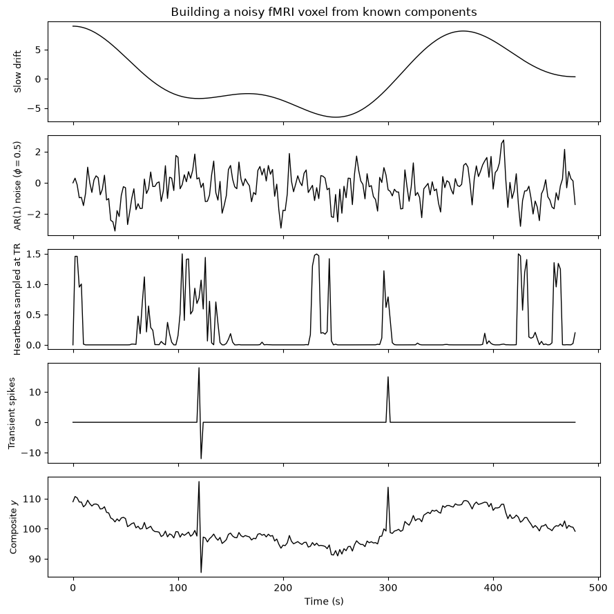
Look at the heartbeat panel: the underlying signal beats once per second, but sampled every 2 s it looks like a slow, irregular wander — nothing like a 1 Hz oscillation. That is temporal aliasing, and Part 2 shows exactly why it happens.
Part 2 — Time and frequency domains, and the aliasing trap
The Fourier transform re-expresses a time series, without loss of information, as a sum of sine waves, each with a magnitude and phase; plotting power against frequency gives the power spectral density (PSD). Sampling imposes a hard limit: by the Nyquist theorem, a sampling rate can only represent frequencies up to
f_Nyquist — highest frequency recoverable from the sampled data (Hz) · F_s — sampling rate, 1/TR (Hz) · TR — repetition time between volumes (s)
where is the highest frequency that can be recovered from the sampled data, the sampling rate, and the repetition time between volumes.
Frequencies above the limit are reflected around it and reappear below — they alias. First, the classic demonstration: a 10 Hz sine wave sampled at only 12 Hz (Nyquist limit 6 Hz) masquerades as a 2 Hz oscillation.
fs_hi, fs_lo, dur, f_sig = 1000, 12, 5, 10   # fast/slow sampling rates (Hz); duration (s); signal frequency (Hz)
tt_hi = np.arange(0, dur, 1 / fs_hi)
tt_lo = np.arange(0, dur, 1 / fs_lo)
x_hi = np.sin(2 * np.pi * f_sig * tt_hi)
x_lo = np.sin(2 * np.pi * f_sig * tt_lo)

f1, p1 = signal.periodogram(x_hi, fs=fs_hi)
f2, p2 = signal.periodogram(x_lo, fs=fs_lo)

fig, (ax0, ax1) = plt.subplots(2, 1, figsize=(9, 6))
ax0.plot(tt_hi, x_hi, "k", lw=0.7, label="10 Hz signal (sampled at 1000 Hz)")
ax0.plot(tt_lo, x_lo, "m.-", lw=1.5, label="same signal sampled at 12 Hz")
ax0.set(xlabel="Time (s)", xlim=(0, 2),
        title="Aliasing of a 10 Hz signal sampled at 12 Hz")
ax0.legend(loc="upper right", fontsize=8)

ax1.plot(f1, p1 / p1.max(), "k", label="original (peak at 10 Hz)")
ax1.plot(f2, p2 / p2.max(), "m", label="sampled at 12 Hz (aliased to 2 Hz)")
ax1.axvline(fs_lo / 2, color="gray", ls=":", label="Nyquist limit (6 Hz)")
ax1.set(xlabel="Frequency (Hz)", ylabel="Normalized power", xlim=(0, 12),
        title="Frequency domain: the peak is reflected around the Nyquist limit")
ax1.legend(fontsize=8)
plt.tight_layout()

print(f"Aliased frequency predicted by reflection: {fs_lo - f_sig} Hz")
Aliased frequency predicted by reflection: 2 Hz
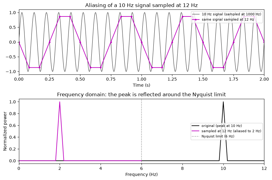
The 10 Hz peak is reflected around the 6 Hz Nyquist limit and lands at 12 − 10 = 2 Hz. Now the version that matters for fMRI: our ~1 Hz heartbeat sampled at TR = 2 s, where the Nyquist limit is 1/(2 × 2) = 0.25 Hz.
f_hb, p_hb = signal.periodogram(hb_hi - hb_hi.mean(), fs=1 / dt)
f_tr, p_tr = signal.periodogram(hb_tr - hb_tr.mean(), fs=1 / TR)
f_y, p_y = signal.periodogram(y - y.mean(), fs=1 / TR)

fig, (ax0, ax1) = plt.subplots(1, 2, figsize=(10, 3.6))
ax0.plot(f_hb, p_hb / p_hb.max(), "k", lw=0.8, label="true heartbeat (~1 Hz)")
ax0.plot(f_tr, p_tr / p_tr.max(), "m", lw=1.2, label="sampled at TR = 2 s")
ax0.axvline(1 / (2 * TR), color="gray", ls=":", label="Nyquist = 0.25 Hz")
ax0.set(xlabel="Frequency (Hz)", ylabel="Normalized power", xlim=(0, 1.6),
        title="Heartbeat: aliased below the Nyquist limit")
ax0.legend(fontsize=8)

ax1.semilogy(f_y[1:], p_y[1:], "k", lw=0.8)
ax1.set(xlabel="Frequency (Hz)", ylabel="Power (log)",
        title="PSD of the composite voxel: drift dominates low frequencies")
plt.tight_layout()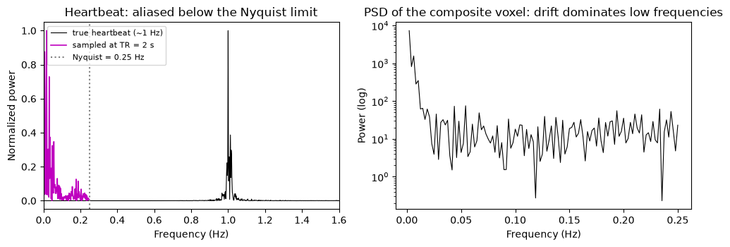
The heartbeat’s power, truly at ~1 Hz, reappears entirely below 0.25 Hz — in the same band as the task and the drift. Because the aliased pattern shifts dramatically with small beat-to-beat timing changes, it cannot be cleanly filtered out or modeled with simple covariates; this is why fast (multiband) sampling or physiological recordings are so valuable.
Part 3 — Detecting transient outliers: RMSSD/DVARS and Mahalanobis distance
Real QC works on whole image volumes, not single voxels. We simulate a small “brain” of 200 voxels sharing drift and heartbeat components (with voxel-specific weights) plus voxel-specific AR(1) noise, and corrupt the same three volumes with spatially widespread intensity shifts.
Two standard diagnostics, both used in CANlab’s scnlab_outlier_id and fmri_data.mahal QC tools:
RMSSD (DVARS) — the root-mean-square change from each image to the next:
RMSSD_t — root-mean-square change from image t−1 to image t · V — number of voxels · y_{v,t} — signal in voxel v at time t
where is the root-mean-square change from image to image , the number of voxels, and the signal in voxel at time .
BOLD changes slowly, so a big image-to-image jump flags a transient artifact.
Mahalanobis distance — how far each image lies from the multivariate cloud of all images (computed here on the first 5 principal components), flagging globally unusual volumes.
V = 200                                        # number of voxels
w_drift = rng.uniform(0.2, 1.5, size=V)        # voxel-specific loadings
w_hb = rng.uniform(0.0, 1.0, size=V)
eta_mat = rng.standard_normal((n, V))
noise = signal.lfilter([1.0], [1.0, -phi], eta_mat, axis=0)

Y = (100 + np.outer(drift, w_drift) + np.outer(1.5 * hb_tr, w_hb) + noise)
Y[spike_vols] += rng.normal(0, 6, size=(len(spike_vols), V))   # corrupt 3 vols

# --- RMSSD / DVARS -------------------------------------------------------
rmssd = np.sqrt(np.mean(np.diff(Y, axis=0) ** 2, axis=1))      # length n-1
z_rmssd = (rmssd - rmssd.mean()) / rmssd.std()
flag_rmssd = np.where(z_rmssd > 3)[0] + 1      # +1: diff t-1 -> t flags t

fig, ax = plt.subplots(figsize=(9, 3.2))
ax.plot(np.arange(1, n), rmssd, "k", lw=0.8)
thresh = rmssd.mean() + 3 * rmssd.std()
ax.axhline(thresh, color="gray", ls="--", label="mean + 3 SD")
ax.plot(flag_rmssd, rmssd[flag_rmssd - 1], "ro", label="flagged volumes")
ax.set(xlabel="Time (images)", ylabel="RMSSD (DVARS)",
       title="Image-to-image change flags the corrupted volumes")
ax.legend(fontsize=8)
plt.tight_layout()

print("True corrupted volumes:", spike_vols)
print("Flagged by RMSSD > 3 SD:", flag_rmssd)
True corrupted volumes: [ 60 61 150]
Flagged by RMSSD > 3 SD: [ 60 61 62 150 151]
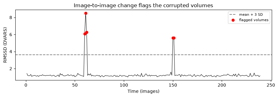
One caution visible in the code: a spike at volume produces large successive differences both into and out of the artifact, so RMSSD may flag the volume after a spike as well. In practice, adjacent flagged volumes are usually all treated as outliers.
Now the multivariate view. We reduce the 200-voxel images to their first 5 principal components and compute each volume’s Mahalanobis distance from the cloud; under approximate normality, squared distances follow a distribution, giving a principled threshold.
Yc = Y - Y.mean(axis=0)
U, s, Vt = np.linalg.svd(Yc, full_matrices=False)
k = 5                                          # number of principal components to keep
scores = U[:, :k] * s[:k]                      # n x k PC scores per volume

Sinv = np.linalg.inv(np.cov(scores, rowvar=False))
d = scores - scores.mean(axis=0)
md2 = np.einsum("ij,jk,ik->i", d, Sinv, d)     # squared Mahalanobis distance

chi2_thresh = stats.chi2.ppf(0.999, df=k)      # expect ~0.1% false flags
flag_mahal = np.where(md2 > chi2_thresh)[0]

fig, ax = plt.subplots(figsize=(9, 3.2))
ax.plot(md2, "k", lw=0.8)
ax.axhline(chi2_thresh, color="gray", ls="--", label="$\chi^2_5$, p < .001")
ax.plot(flag_mahal, md2[flag_mahal], "ro", label="flagged volumes")
ax.set(xlabel="Time (images)", ylabel="Mahalanobis $d^2$",
       title="Multivariate distance from the cloud of images")
ax.legend(fontsize=8)
plt.tight_layout()

print("Flagged by Mahalanobis:", flag_mahal)
Flagged by Mahalanobis: [ 60 61 150]
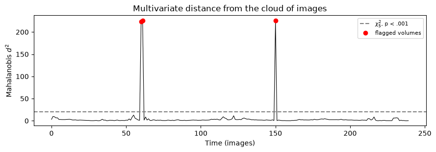
Finally, we handle the outliers the recommended way — not by deleting time points, but by adding one spike regressor per flagged volume to the design matrix. Each regressor is 1 at its bad volume and 0 elsewhere, which removes that image’s influence on the fit while preserving the timing and noise structure of the series. (Deleting time points changes the noise properties, forces re-timing of the design, and can bias sampling when outliers are task-correlated.)
flagged = np.unique(np.concatenate([flag_rmssd, flag_mahal]))
spike_regs = np.zeros((n, len(flagged)))
spike_regs[flagged, np.arange(len(flagged))] = 1.0

print(pd.DataFrame({
    "volume": flagged,
    "true outlier": np.isin(flagged, spike_vols),
    "RMSSD flag": np.isin(flagged, flag_rmssd),
    "Mahalanobis flag": np.isin(flagged, flag_mahal),
}).to_string(index=False))
print("\nSpike regressor matrix shape:", spike_regs.shape,
      "-> add these columns to the design matrix X")
volume true outlier RMSSD flag Mahalanobis flag
60 True True True
61 True True True
62 False True False
150 True True True
151 False True False
Spike regressor matrix shape: (240, 5) -> add these columns to the design matrix X
Part 4 — Autocorrelation and its consequences for naive OLS
Even after drift removal and outlier handling, fMRI noise remains autocorrelated. For AR(1) noise, the theoretical autocorrelation function (ACF) decays geometrically: . Let’s check the empirical ACF of our noise against theory.
e = signal.lfilter([1.0], [1.0, -phi], rng.standard_normal(5000))  # long AR(1) sample for stable estimates
max_lag = 15                              # longest lag (in TRs) to examine
acf = np.array([1.0] + [np.corrcoef(e[:-k], e[k:])[0, 1]
                        for k in range(1, max_lag + 1)])

fig, ax = plt.subplots(figsize=(7, 3.4))
ax.stem(np.arange(max_lag + 1), acf, basefmt="gray", label="empirical ACF")
ax.plot(np.arange(max_lag + 1), phi ** np.arange(max_lag + 1), "r.-",
        lw=1, label=r"theoretical $\phi^k$")
ax.set(xlabel="Lag (TRs)", ylabel="Correlation",
       title="Autocorrelation function of AR(1) noise, $\phi = 0.5$")
ax.legend(fontsize=9)
plt.tight_layout()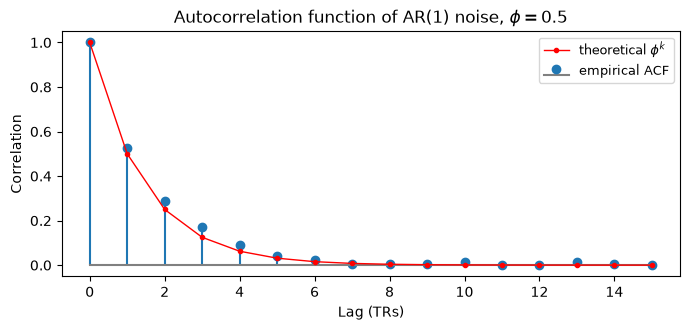
Why does this matter? OLS standard errors assume independent errors. Positively autocorrelated noise contains fewer effectively independent observations than time points, so OLS underestimates the variability of — and t-statistics are inflated.
To see it, we run a null simulation: fit a blocked task regressor (40 s on/off) to pure AR(1) noise containing no signal whatsoever, 2,000 times, and count how often naive OLS declares p < .05. If inference were valid, the answer would be ~5%. Then we repeat after prewhitening — transforming both and so the errors become independent (here using the known ; real software estimates it from residuals, per Chapter 19).
nsim = 2000                               # number of null simulations; more for stable tail estimates
Xd = np.c_[(np.sin(2 * np.pi * t / 80) > 0).astype(float), np.ones(n)]
p_ = Xd.shape[1]
tcrit = stats.t.ppf(0.975, n - p_)

# Generate all null datasets at once: pure AR(1) noise, no signal
E = signal.lfilter([1.0], [1.0, -phi],
                   rng.standard_normal((n, nsim)), axis=0)

def ols_fpr(X, E):
    B = np.linalg.lstsq(X, E, rcond=None)[0]        # p x nsim
    R = E - X @ B
    s2 = np.sum(R ** 2, axis=0) / (n - X.shape[1])
    c00 = np.linalg.inv(X.T @ X)[0, 0]
    tvals = B[0] / np.sqrt(s2 * c00)
    return np.mean(np.abs(tvals) > tcrit)

fpr_naive = ols_fpr(Xd, E)

# Prewhitening: W removes AR(1) dependence (exact transform for known phi)
W = np.eye(n) - phi * np.eye(n, k=-1)
W[0, 0] = np.sqrt(1 - phi ** 2)
fpr_white = ols_fpr(W @ Xd, W @ E)

print(f"False positive rate, naive OLS on AR(1) noise: {fpr_naive:.3f}")
print(f"False positive rate after prewhitening:        {fpr_white:.3f}")
print(f"Nominal rate: 0.050")
False positive rate, naive OLS on AR(1) noise: 0.221
False positive rate after prewhitening: 0.051
Nominal rate: 0.050
Naive OLS produces several times too many false positives — every one of them a “significant activation” in data containing no signal at all. Prewhitening restores the nominal 5% rate. This is exactly why fMRI software estimates the noise autocorrelation and applies generalized least squares (prewhitening) at the first level, as developed in Chapters 18–19.
Wrap-up
fMRI noise is structured: slow drift (1/f), autocorrelated AR-like noise, transient spikes, and physiological components that alias when sampled at the TR.
The Nyquist limit determines which physiological frequencies survive sampling intact; a 1 Hz heartbeat sampled at TR = 2 s becomes unpredictable low-frequency noise.
RMSSD/DVARS and Mahalanobis distance are complementary outlier detectors; flagged volumes are best handled with spike regressors, not deletion.
Autocorrelation inflates naive OLS t-statistics; prewhitening (GLS) restores valid inference.
The MATLAB version of this lab mirrors these steps with CANlab tools (noise_arp, scnlab_outlier_id, fmri_data.mahal).