Group Analysis
Run this code: ⚡ In-browser lab · Colab · MATLAB Online
Overview
The previous chapters fit GLMs to one person’s time series. But science is ultimately about generalizable knowledge: most studies aim to draw conclusions about a population of unobserved individuals, not about the particular people who happened to be scanned. That requires group analysis — combining results across multiple subjects performing the same type of experiment. Like single-subject analysis, group analysis is typically mass univariate: each voxel (after normalization to a common template space, Chapter 17) is regressed on task or behavioral variables, and the same inferential test is repeated across the brain.
Multi-subject fMRI data are fundamentally hierarchical: volumes are nested within runs, runs within sessions, sessions within subjects, and subjects within groups. Task effects on brain activity are assessed within-person, while group differences and individual-difference variables (age, sex, behavioral performance, patient vs. control) are assessed between-person. Group analyses respect this structure with a two-level hierarchical model: the first level estimates within-subject effects for each individual, and the second level analyzes those effects across subjects to test (a) whether within-person effects generalize to the population and (b) whether they are moderated by person-level variables.
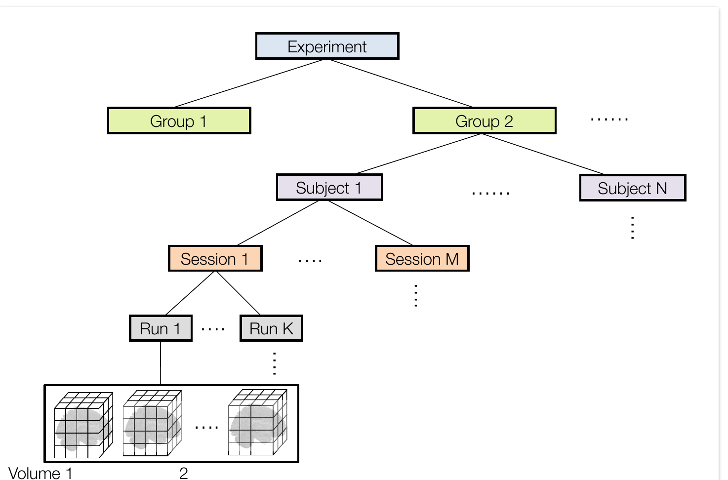
The hierarchical structure of fMRI data. Brain volumes are nested within runs, runs within sessions, sessions within subjects, and subjects within groups. Within-person effects (tasks) and between-person effects (group, individual differences) live at different levels of this hierarchy. (Figure 12.8 from the book. © the authors and MIT Press; reproduced with permission — not covered by this site’s CC-BY license.)
The workhorse implementation is the summary statistics approach. A first-level GLM is fit separately to each subject, producing a contrast image — a Contrast of Parameter Estimates (COPE) map, e.g., for [Task A − Task B] — for each effect of interest. These per-subject contrast values then become the outcome data for a second-level GLM at each voxel. The simplest second-level model contains only an intercept, which tests whether the mean contrast differs from zero across participants: a one-sample t-test at every voxel. Richer second-level models add predictors such as group membership, age, sex, or behavioral performance, whose maps test whether those variables moderate the within-person effect.
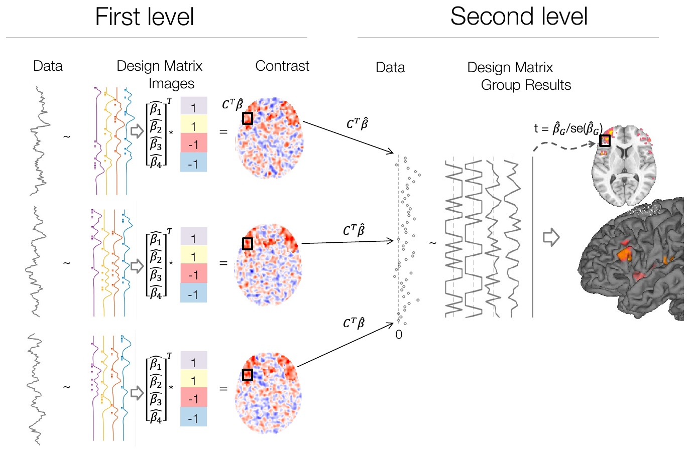
The summary statistics approach to group analysis. A first-level GLM is fit separately to each subject and contrast images (, where is a contrast vector and the estimated first-level coefficients) are created. At the second level, the per-subject contrast values are the data for a group model — e.g., a one-sample t-test on whether the contrast differs from 0 — yielding a group statistic map. (Figure 21.1 from the book. © the authors and MIT Press; reproduced with permission — not covered by this site’s CC-BY license.)
This procedure is often called a random effects analysis because it treats subject as a random effect: the group mean is compared against inter-subject variability. The name arose in contrast to early fixed effects analyses, which concatenated all subjects’ data into one “super subject” and fit a single model, assuming the only source of error is within-subject measurement noise. A fixed-effects analysis technically supports inferences about the specific people scanned, but not about anyone else — and such non-generalizable conclusions are seldom useful in any field. The labels are somewhat misleading, though: fixed and random effects are not types of analysis but ways of modeling variability. Fixed effects are variables whose specific levels are theoretically meaningful — drug vs. placebo, Task A vs. B, male vs. female. Random effects are variables whose levels are sampled from a population we want to generalize over; subject is the quintessential random effect.
Formally, the first-level GLM for subject , where indexes the subjects in the study, is
yᵢ — subject i’s fMRI time series (time × 1) · Xᵢ — subject i’s design matrix (time × predictors) · βᵢ — subject-specific regression parameters · εᵢ — within-subject measurement noise · m — number of subjects
where is the fMRI time-series vector for subject , that subject’s design matrix (time points × predictors), the subject-specific regression parameters, within-subject measurement noise, and the number of subjects.
and the second level models the subject-specific parameters as random draws around group parameters:
βᵢ — subject-specific parameters · Z_G — second-level (group) design matrix · β_G — population effects · ηᵢ — subject i’s deviation from the group values · U_G — covariance of the random effects
where is the second-level design matrix (e.g., intercept plus group or covariate columns), the vector of population effects, subject ’s random deviation from those group values, and the covariance matrix of the random effects — the variances (and covariances) of true individual differences.
Substituting the second level into the first gives a single-level form whose composite error contains both variance components: the within-subject covariance (from ) plus the between-subject covariance (from ). A correctly specified mixed effects model estimates both components — typically by restricted maximum likelihood (ReML) with iterative algorithms such as EM — and weights each subject’s contribution in proportion to its precision (inverse variance), so noisier subjects influence the group estimate less. The summary statistics approach implicitly treats subject as a random effect: because each subject contributes one number per voxel, variation across those numbers is the between-subject error term. When first-level standard errors are equal across subjects, the simple two-stage approach is valid and fully efficient — as powerful as the full mixed model.
In practice the summary statistics approach dominates fMRI (nearly 90% of papers): it is valid, computationally cheap, and combines naturally with robust regression, bootstrapping, and permutation tests. Simulation studies have found it surprisingly robust, with appropriate false positive control and near-optimal power under typical designs. Full mixed models are slower and easier to misuse, but they are more powerful for complex designs — longitudinal and twin studies, missing data, and variable data quality across people. Software occupies a spectrum of compromises, many using precision-weighted summary statistics: FSL’s FLAME, AFNI’s 3dMEMA, SPM’s spm_mfx, and CANlab’s igls.m / glmfit_multilevel.m among others.
Three practical issues can dramatically change group results. Masking: many packages silently drop voxels missing in any subject or with low signal, so group maps can omit swaths of cortex; use explicit masks and check group-level coverage. Second-level covariates: adding a mean-centered performance covariate (or effects-coded sex, order, etc.) can increase power for the group-average effect by removing known between-person variance — but the intercept’s meaning now depends on where zero falls for every covariate, so centering and coding choices matter. Outliers: with tens of thousands of voxels, extreme values are inevitable and hard to inspect by hand; a single outlier subject can flip a slope’s sign or manufacture significance. Robust regression — iteratively reweighted least squares (IRLS) — automatically down-weights outlying observations, costing a little power when there are no true outliers and gaining substantial power when there are.
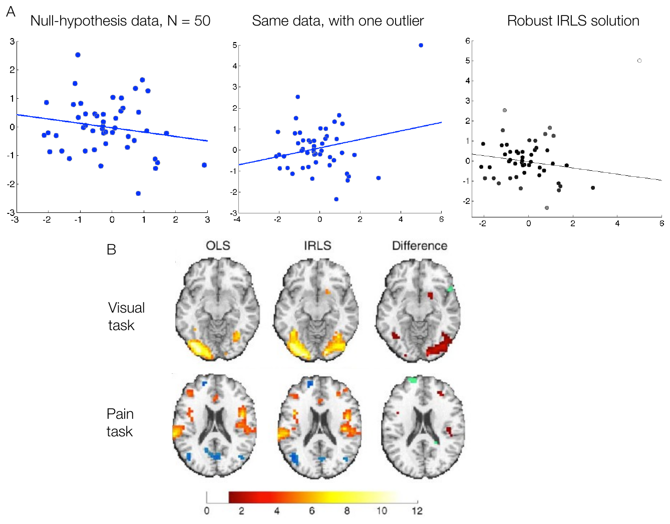
Outliers and robust regression. (A) In null-hypothesis data (, left), adding a single extreme point (center) flips the estimated slope and makes the correlation spuriously significant. The robust IRLS solution (right) automatically down-weights the outlier (open circle; lighter shading = lower weight). (B) Compared with OLS, IRLS yields stronger group activation in visual cortex for a visual task and contralateral somatosensory regions for a pain task. (Figure 21.4 from the book. © the authors and MIT Press; reproduced with permission — not covered by this site’s CC-BY license.)
Hands-on tutorial
In this tutorial you will simulate hierarchical (multi-subject) data with known ground truth, then see for yourself why the analysis choices above matter: a fixed-effects analysis produces wildly inflated false positive rates when subjects truly vary, while the summary statistics (random effects) approach stays honest — and a robust group fit shrugs off an outlier subject that fools OLS.
Step 1 — Fixed vs. random effects inference. We simulate 20 subjects × 40 trials with zero true group effect but real between-subject variability, then test the group effect two ways: pooling all trials as if they came from one super subject (FFX), and a one-sample t-test on subject means (RFX / summary statistics). Run it repeatedly and count false positives.
% Simulate hierarchical null data: true group mean = 0, but subjects differ
rng(7);                        % seed the random number generator for reproducibility
n_subj = 20; n_trials = 40;    % n_subj = subjects, n_trials = trials per subject
sigma_between = 0.5;           % SD of true subject effects (real individual differences)
sigma_within  = 1.0;           % SD of trial-level (within-subject) noise

n_iter = 1000;                 % number of simulated experiments; more -> stabler FPR estimate
p_ffx = zeros(n_iter, 1); p_rfx = zeros(n_iter, 1);   % p-values per experiment
for it = 1:n_iter
    subj_fx = sigma_between .* randn(n_subj, 1);            % eta_i
    Y = repmat(subj_fx', n_trials, 1) + sigma_within .* randn(n_trials, n_subj);
    [~, p_ffx(it)] = ttest(Y(:));                           % FFX: pool all trials
    [~, p_rfx(it)] = ttest(mean(Y)');                       % RFX: subject means
end
fprintf('False positive rate at alpha = .05:  FFX = %.3f   RFX = %.3f\n', ...
    mean(p_ffx < .05), mean(p_rfx < .05))
import numpy as np
from scipy import stats
rng = np.random.default_rng(7) # seed for reproducibility
n_subj, n_trials = 20, 40 # n_subj = subjects, n_trials = trials per subject
sigma_between, sigma_within = 0.5, 1.0 # between-subject SD, trial-level noise SD
n_iter, p_ffx, p_rfx = 1000, [], [] # n_iter = simulated experiments; more -> stabler FPR
for _ in range(n_iter):
subj_fx = sigma_between * rng.standard_normal(n_subj) # eta_i
Y = subj_fx + sigma_within * rng.standard_normal((n_trials, n_subj))
p_ffx.append(stats.ttest_1samp(Y.ravel(), 0).pvalue) # FFX: pool
p_rfx.append(stats.ttest_1samp(Y.mean(axis=0), 0).pvalue) # RFX: means
print(f"False positive rate at alpha = .05: "
f"FFX = {np.mean(np.array(p_ffx) < .05):.3f} "
f"RFX = {np.mean(np.array(p_rfx) < .05):.3f}")Example output:
False positive rate at alpha = .05: FFX = 0.514 RFX = 0.045The FFX test rejects the (true) null on a large fraction of runs — its error term omits between-subject variance, so its standard errors are far too small — while the RFX false positive rate stays near the nominal 5%.
Step 2 — OLS vs. robust regression with an outlier subject. At the second level, each subject contributes one contrast value, and we relate it to a covariate (e.g., behavioral performance). One outlier subject can reverse the OLS slope; a robust IRLS fit down-weights it automatically.
% Second-level data: one COPE per subject + covariate; no true relationship
rng(11);                                    % seed for reproducibility
n_subj = 30;                                % subjects contributing one COPE each
perf = randn(n_subj, 1);                    % behavioral covariate (mean-centered)
cope = 0.3 .* randn(n_subj, 1);             % contrast values; true slope = 0
perf(end) = 4; cope(end) = 3;               % make the last subject an extreme outlier

b_ols = glmfit(perf, cope);                                  % OLS fit
[b_rob, stat] = robustfit(perf, cope);                       % IRLS (bisquare)
fprintf('Slope:  OLS = %.3f   robust = %.3f\n', b_ols(2), b_rob(2))
fprintf('Robust weight for outlier subject: %.3f\n', stat.w(end))
% CANlab robfit.m / robust_results_batch apply this voxelwise to images
import numpy as np, statsmodels.api as sm
rng = np.random.default_rng(11) # seed for reproducibility
n_subj = 30 # subjects contributing one COPE each
perf = rng.standard_normal(n_subj) # behavioral covariate (mean-centered)
cope = 0.3 * rng.standard_normal(n_subj) # contrast values; true slope = 0
perf[-1], cope[-1] = 4, 3 # make the last subject an extreme outlier
X = sm.add_constant(perf)
b_ols = sm.OLS(cope, X).fit() # OLS fit
b_rob = sm.RLM(cope, X, M=sm.robust.norms.TukeyBiweight()).fit() # IRLS
print(f"Slope: OLS = {b_ols.params[1]:.3f} robust = {b_rob.params[1]:.3f}")
print(f"Robust weight for outlier subject: {b_rob.weights[-1]:.3f}")Example output:
Slope:  OLS = 0.281   robust = -0.036
Robust weight for outlier subject: 0.000
The full labs go further: they visualize the hierarchy of within- and between-subject variance, compare FFX and RFX degrees of freedom and standard errors on a single dataset, fit a genuine mixed effects model (random intercepts and slopes) to trial-level data, and map how the robust weight given to the outlier shrinks as it moves farther from the central mass.
Open the full Python lab notebook → or download the MATLAB live script, which mirrors it using CANlab tools (glmfit_multilevel, fitlme, robustfit).


Thought questions
A colleague argues that because a fixed-effects “super subject” analysis uses every time point from every person, it is more powerful and therefore better. Construct a careful reply: what exactly does the FFX error term omit, what population do FFX inferences apply to, and under what (rare) circumstances might an FFX analysis be defensible?
The one-sample t-test on contrast images is “valid and fully efficient if the standard errors of contrast estimates are the same for all subjects.” Describe three realistic ways this homogeneity assumption fails in an fMRI study, and explain how a precision-weighted mixed model changes each subject’s influence on the group result in response.
In a study of working memory, you can test group-average activation with an intercept-only model or with a model that also includes mean-centered behavioral performance. Explain how adding the covariate can make the intercept test more significant, and how a failure to center (or an effects-coding mistake for sex) could change what the intercept even means.
Robust regression down-weights outlying subjects automatically, but an “outlier” might be a scanner artifact — or a genuinely different brain. Discuss how you would distinguish these cases, what down-weighting implies for the population you are generalizing to in each case, and whether the answer should differ for patient studies.
Mixed effects models are more powerful for longitudinal and twin designs but slower and easier to misspecify. For a four-year longitudinal intervention study with dropout (missing sessions), sketch the second-level model you would fit — which effects are fixed, which random — and argue whether the summary statistics approach could still be made to work.
Quiz yourself
Q1. In the two-level summary statistics approach, what happens at each level?
Answer: At the first level, a GLM is fit separately to each subject’s time series, producing contrast (COPE) images for each effect of interest. At the second level, those per-subject contrast values become the outcome data in a group GLM at each voxel — in the simplest case, a one-sample t-test on whether the mean contrast differs from zero.
Q2. Define fixed and random effects, and give an example of each in a typical fMRI study.
Answer: Fixed effects are variables whose specific levels are theoretically meaningful — e.g., Task A vs. Task B, drug vs. placebo, or sex. Random effects are variables whose levels are randomly sampled from a population we want to generalize over — subject is the quintessential example, since each participant is one draw from the population of interest.
Q3. Why is a fixed-effects (“super subject”) analysis inappropriate for population inference?
Answer: It assumes the only source of error is within-subject measurement noise, omitting true differences between individuals from the error term. Its inferences therefore apply only to the specific subjects scanned, and if between-subject variability exists, its standard errors are too small and false positive rates are inflated for any population-level claim.
Q4. What are the two variance components a correctly specified mixed effects model estimates, and how do they enter the group-level error?
Answer: (1) Within-subject measurement error (including model misfit), and (2) between-subject variance — the variance of the random subject effects. The composite error covariance of the group model contains both, so inference on group effects accounts for measurement noise and true individual differences.
Q5. How does a precision-weighted mixed model treat a subject whose first-level estimates are noisy (large standard errors)?
Answer: Each subject’s contribution to the group estimate is weighted in proportion to the precision (inverse variance) of that subject’s estimate. A subject with large first-level standard errors is less reliable and is therefore down-weighted, improving power when data quality varies across people.
Q6. When is the simple one-sample t-test on contrast images just as powerful as a full mixed effects model?
Answer: When the standard errors of the first-level contrast estimates are (approximately) equal across subjects — homogeneous within-person efficiency. Under that condition the summary statistics approach is valid and fully efficient, which helps explain why nearly 90% of fMRI studies use it.
Q7. You add a behavioral performance covariate and effects-coded sex (−1/1) to a second-level model. What does the intercept test if performance is mean-centered — and if it is not?
Answer: The intercept is the expected contrast value when all covariates equal zero. With mean-centered performance and effects-coded sex, it reflects the group-average activation at average performance, at the midpoint of the sexes. If performance is not centered, the intercept instead reflects predicted activation at a performance score of zero — possibly far outside the observed range — changing both its significance and its meaning.
Q8. What does robust (IRLS) regression do, and what is the cost–benefit tradeoff relative to OLS?
Answer: It iteratively reweights observations, down-weighting points that lie far from the fit of the central mass of the data, so outliers cannot dominate the estimate. If no true outliers exist it costs a modest amount of power; when outliers are present it protects against spurious or masked effects and can substantially improve power in group fMRI analyses.
 The book: Elements of Functional Magnetic Resonance Imaging — Wager & Lindquist, MIT Press