Multiple Comparisons
Run this code: ⚡ In-browser lab · Colab · MATLAB Online
Overview
A standard fMRI analysis produces a statistical map: a t (or z, or F) value at every voxel, testing an effect of interest at that location. A standard 2 × 2 × 2 mm brain mask contains roughly 240,000 voxels — which means roughly 240,000 simultaneous hypothesis tests. If we simply declared every voxel with “active,” we would expect about 5% of truly null voxels to cross that threshold by chance: on the order of 12,000 false positive voxels in a single map. The choice of threshold therefore has an enormous impact on which voxels are deemed active, as Figure 22.1 shows, and correcting for multiplicity is essential for meaningful inference.
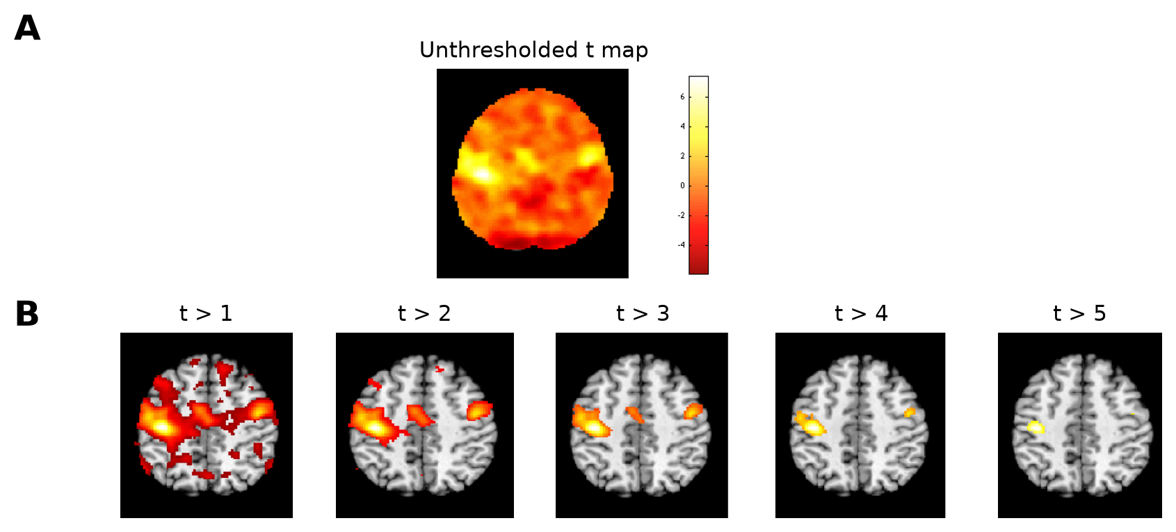
Figure 1:Thresholding at different levels. (A) A t statistic image from a group analysis, with a separate hypothesis test at each voxel. (B) The same image thresholded at five increasingly stringent values; voxels deemed significant are color-coded on an anatomical underlay. The choice of threshold has a large impact on which voxels are deemed active. (Figure 22.1 from the book. © the authors and MIT Press; reproduced with permission — not covered by this site’s CC-BY license.)
Two families of corrections dominate neuroimaging. Procedures that control the family-wise error rate (FWER) limit the probability of obtaining any false positives anywhere in the map. Procedures that control the false discovery rate (FDR) instead limit the expected proportion of false positives among the voxels declared significant. A second, orthogonal choice is the level of inference: voxelwise inference treats each voxel as the unit of analysis, whereas clusterwise inference asks whether groups of contiguous suprathreshold voxels are larger than expected by chance.
The simplest FWER procedure is Bonferroni correction: to control FWER at level across tests — where is the Type I error rate you are willing to tolerate for the whole family (e.g., 0.05) and is the number of tests — threshold each test at
α_per test — significance threshold applied to each individual test · α — family-wise Type I error rate to be controlled (e.g., 0.05) · m — number of simultaneous tests (voxels)
where is the threshold applied to each individual test, the family-wise Type I error rate to be controlled, and the number of simultaneous tests.
With tests and , each voxel must reach . Because fMRI data are spatially smooth — neighboring voxels are highly correlated, and smoothing during preprocessing adds more correlation — the effective number of independent tests is far smaller than the number of voxels, and Bonferroni is unnecessarily conservative. Random Field Theory (RFT) addresses this by treating the statistical map as a discrete sample of a smooth random field. Using the image’s estimated smoothness (expressed in resolution elements, or resels) and a topological property called the Euler characteristic, RFT computes the probability that any voxel (or any cluster of a given size) exceeds a threshold under the null — a closed-form FWER threshold that adapts to the smoothness of the data. RFT tends to be conservative for voxelwise inference in small samples, however, and — critically — too liberal for clusterwise inference when the cluster-defining threshold is lenient.
Clusterwise inference itself is a two-step procedure: threshold the map at a primary (“cluster-defining”) threshold, then test whether each resulting cluster’s extent (number of contiguous voxels) exceeds what chance would produce. It is on average more sensitive than voxelwise inference and became the dominant approach in the literature, but it comes with serious caveats. The significance statement applies to the cluster as a whole: rejecting the null of “no signal anywhere in the cluster” licenses only the conclusion that there is signal somewhere in the cluster — not that any particular voxel, or even any particular region, is active. With liberal primary thresholds (e.g., ), clusters often sprawl across many anatomical regions, degrading spatial interpretability, and parametric cluster corrections become invalid, inflating false positives well above their nominal rate. Threshold-free cluster enhancement (TFCE) sidesteps the arbitrary primary threshold by integrating cluster extent over all possible thresholds:
TFCE(v) — enhanced statistic at voxel v · h — cluster-forming threshold (variable of integration) · h₀ — lowest threshold considered · h_v — statistic value at voxel v · e(h) — extent of the cluster containing v at threshold h · E, H — extent and height weights (typically E = 0.5, H = 2)
where sweeps over cluster-forming thresholds from up to the voxel’s own statistic value , is the extent of the cluster containing voxel at threshold , and the exponents and (typically 0.5 and 2) weight extent against height.
The result retains cluster-level sensitivity without committing to a single cluster-defining height.
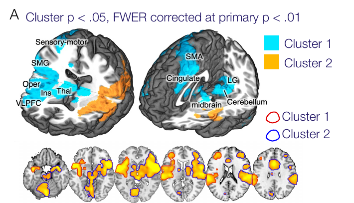
Figure 2:Cluster extent-based thresholding and its limitations. In an analysis of pain-related activity, a liberal primary threshold ( uncorrected) yields widespread activation that forms two clusters significant by FWER-corrected cluster extent (, outlined). The valid inference is only that each cluster contains at least one truly active voxel somewhere within it — the true activation could lie in many different structures, and a substantial fraction of the colored voxels are expected to be false discoveries. (Panel A of Figure 22.2 from the book. © the authors and MIT Press; reproduced with permission — not covered by this site’s CC-BY license.)
The Benjamini–Hochberg (BH) procedure is the FDR-controlling method used almost universally in fMRI. Choose an FDR level (e.g., 0.05) — the expected proportion of false discoveries you are willing to tolerate, written rather than to signal that a different error rate is being controlled — rank the p-values from smallest to largest, , and find the largest rank such that
p(r) — the r-th smallest p-value · r — rank in the sorted list · m — number of tests · q — chosen FDR level (e.g., 0.05)
where is the -th smallest p-value, the number of tests, and the chosen FDR level.
All tests with are declared significant. The procedure is adaptive: the more signal in the map, the more small p-values there are, and the lower (more generous) the resulting threshold. Because it operates on p-values alone, BH can be wrapped around any valid statistical test.
How do the two philosophies compare? Under a pure null — no true signal anywhere — the two criteria coincide: every rejection is a false discovery, so FDR control is equivalent to FWER control, and a properly corrected map should produce a false positive in only about 1 of 20 experiments at the 5% level. When true signal is present, any FWER-controlling procedure also controls FDR, so FDR control is necessarily less stringent — and more powerful. Suppose tests on 100,000 voxels at uncorrected yield 300 “significant” voxels, of which roughly 100 are expected to be false positives — a third of the discoveries, with no way to tell which. FDR control at instead sets the threshold so that only about 5% of reported voxels are expected to be false discoveries, letting us argue that most reported results are real. FWER control at 5% is stronger still — only 5 in 100 repeated experiments would yield any false positive voxel — but the price is a stringent threshold that can miss most of the truly active voxels, trading Type I errors for a large increase in Type II errors.
Nonparametric permutation methods use the data itself to build the null distribution, requiring only exchangeability under the null (for group analyses, subjects are typically exchangeable; individual time points are not, because of temporal autocorrelation). To control FWER, one recomputes the statistic map under many relabelings (e.g., sign flips of subject contrast images for a one-sample test), records the maximum statistic across the brain in each relabeling, and thresholds the observed map at the 95th percentile of this max distribution. Because whole images are resampled together, spatial dependence is handled automatically — no smoothness model required. Permutation approaches are computationally intensive but are widely regarded as the gold standard, providing accurate false positive control where parametric cluster methods fail; tools such as FSL’s randomise and PALM extend them to general designs with nuisance covariates.
Finally, a practical note. Many published studies still report arbitrary uncorrected thresholds (e.g., ), largely because corrected thresholds combined with small samples leave power extremely low — but uncorrected maps from individual studies should not be strongly interpreted; they are best reserved for archival purposes and meta-analysis. A complementary strategy is to reduce the family of tests in the first place: pre-specify a small number of regions of interest, network averages, or multivariate pattern responses, and report all of them, significant or not. When even that family grows large, one can test whether the number of positive results exceeds what chance would produce under a global null. Choosing a correction is ultimately a choice about which errors you can afford — and being explicit about that choice is part of doing honest science.
Hands-on tutorial
The multiple comparisons problem is easy to experience for yourself with simulation — no brain data required. We will generate thousands of statistical tests where we know the ground truth, and watch what different corrections do. The MATLAB versions run in base MATLAB with the Statistics and Machine Learning Toolbox; the Python versions need only NumPy, SciPy, Matplotlib, and statsmodels.
1. Manufacture false positives: 10,000 null tests
Simulate a “brain” of 10,000 voxels in which nothing is truly active — 30 subjects of pure noise — and run a one-sample t-test at every voxel.
% 10,000 tests, all null: n = 30 subjects, no true effect anywhere
% (Adapted from FMRI_simulations/statistical_principles by Tor Wager)
rng(42);         % seed the random-number generator for reproducibility
n = 30;          % n = subjects
k = 10000;       % k = number of tests (voxels)

dat = randn(n, k);            % pure noise
[~, p] = ttest(dat);          % one-sample t-test at each voxel

nsig = sum(p < .05);
fprintf('%d of %d null tests are "significant" at p < .05 (expected ~%d)\n', ...
    nsig, k, .05 * k);

% Where are they? Salt-and-pepper false positives across the "brain"
imagesc(reshape(p < .05, 100, 100)); axis image; colormap(gray)
title('False positives at p < .05, pure noise')
# 10,000 tests, all null: n = 30 subjects, no true effect anywhere
import numpy as np
from scipy import stats
import matplotlib.pyplot as plt
rng = np.random.default_rng(42) # seed for reproducibility
n, k = 30, 10000 # n = subjects, k = number of tests (voxels)
dat = rng.standard_normal((n, k)) # pure noise
t, p = stats.ttest_1samp(dat, 0) # one-sample t-test at each voxel
nsig = (p < .05).sum()
print(f'{nsig} of {k} null tests are "significant" at p < .05 '
f'(expected ~{int(.05 * k)})')
# Where are they? Salt-and-pepper false positives across the "brain"
plt.imshow((p < .05).reshape(100, 100), cmap='gray')
plt.title('False positives at p < .05, pure noise')
plt.show()Example output:
529 of 10000 null tests are "significant" at p < .05 (expected ~500)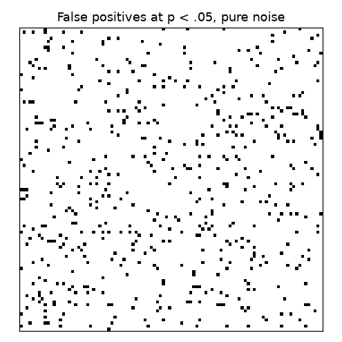
False positives at across 10,000 pure-noise tests, arranged as a 100 × 100 “slice.”
You should see roughly 500 “significant” voxels — every one of them a false positive, scattered salt-and-pepper across the image. This is exactly what an uncorrected map of a null contrast looks like. Apply a valid FWER correction to this same null map, and any false positive at all should appear in only ~1 of 20 repeated runs — and because under a pure null every rejection is a false discovery, FDR control here is equivalent to FWER control: almost nothing survives either correction.
2. Bonferroni and FDR with real signal present
Now plant true effects in 10% of tests (Cohen’s , ) and compare uncorrected, Bonferroni, and Benjamini–Hochberg thresholds on sensitivity and false discoveries.
% Signal in 10% of tests: d = 0.5, n = 50
% (Adapted from fdr_sims_playground.m, FMRI_simulations repo, Tor Wager)
rng(7);                                 % seed for reproducibility
n = 50;  k = 10000;  d = 0.5;           % n = subjects, k = tests, d = true effect size (Cohen's d)
numtrue = k / 10;                       % 1,000 truly active tests (10%)
mu = [d * ones(1, numtrue), zeros(1, k - numtrue)];

dat = mu + randn(n, k);
[~, p] = ttest(dat);

% Benjamini-Hochberg step-up: largest r with p(r) <= (r/k)*q
q = 0.05;                                % FDR level: tolerated proportion of false discoveries
psort = sort(p);
r = find(psort <= (1:k) / k * q, 1, 'last');
p_fdr = psort(r);                        % BH threshold
% With CANlab Core on your path: p_fdr = FDR(p, .05);

thresholds = [.05, .05/k, p_fdr];        % uncorrected, Bonferroni, FDR
names = {'Uncorrected', 'Bonferroni', 'FDR (BH)'};
istrue = (1:k) <= numtrue;
for i = 1:3
    sig = p < thresholds(i);
    tpr = sum(sig & istrue) / numtrue;              % sensitivity
    fdr_obs = sum(sig & ~istrue) / max(sum(sig), 1); % observed FDR
    fprintf('%-12s thresh %.2g: %4d sig, TPR %.2f, observed FDR %.3f\n', ...
        names{i}, thresholds(i), sum(sig), tpr, fdr_obs);
end
# Signal in 10% of tests: d = 0.5, n = 50
import numpy as np
from scipy import stats
from statsmodels.stats.multitest import multipletests
rng = np.random.default_rng(7) # seed for reproducibility
n, k, d = 50, 10000, 0.5 # n = subjects, k = tests, d = true effect size (Cohen's d)
numtrue = k // 10 # 1,000 truly active tests (10%)
mu = np.r_[d * np.ones(numtrue), np.zeros(k - numtrue)]
dat = mu + rng.standard_normal((n, k))
t, p = stats.ttest_1samp(dat, 0)
# Benjamini-Hochberg step-up: largest r with p(r) <= (r/k)*q; alpha here is q, the FDR level
rej_fdr = multipletests(p, alpha=0.05, method='fdr_bh')[0]
p_fdr = p[rej_fdr].max() if rej_fdr.any() else 0.0 # BH threshold
istrue = np.arange(k) < numtrue
for name, sig in [('Uncorrected', p < .05),
('Bonferroni', p < .05 / k),
('FDR (BH)', rej_fdr)]:
tpr = (sig & istrue).sum() / numtrue # sensitivity
fdr_obs = (sig & ~istrue).sum() / max(sig.sum(), 1) # observed FDR
print(f'{name:<12s}: {sig.sum():4d} sig, TPR {tpr:.2f}, '
f'observed FDR {fdr_obs:.3f}')Example output:
Uncorrected : 1362 sig, TPR 0.93, observed FDR 0.316
Bonferroni  :   87 sig, TPR 0.09, observed FDR 0.000
FDR (BH)    :  694 sig, TPR 0.67, observed FDR 0.037
Compare the three rows: uncorrected finds the most true effects but ~30–50% of its discoveries are false; Bonferroni makes almost no false discoveries but misses most of the real signal; BH-FDR sits in between, keeping the false fraction near 5% while retaining much of the sensitivity. The full labs visualize the BH ranked-p threshold line, repeat the simulation to see the variability of the observed FDR, and build a permutation max-t FWER threshold from scratch.
Open the full Python lab notebook → or download the MATLAB live script.
Thought questions
A colleague reports a cluster of 4,000 voxels spanning insula, operculum, and putamen, significant at cluster-corrected with a primary threshold of , and concludes that “the insula was activated.” What can they validly conclude, and how would you redesign the analysis to support a claim about the insula specifically?
FDR control at and FWER control at can both be described as “5% error control,” yet they license very different statements about a thresholded map. For a study intended to guide neurosurgical planning versus an exploratory mapping study, which criterion would you choose for each, and why?
Bonferroni correction becomes more conservative as the correlation among tests increases, yet spatial smoothing — which increases correlation among voxels — is standard practice. How do these two facts interact when choosing a correction strategy, and how do RFT and permutation approaches each exploit smoothness?
The BH procedure is adaptive: with more true signal in the map, its threshold becomes more liberal. Explain why this adaptivity does not break its control of the false discovery rate, and describe a scenario (drawing on the simulation results) where the observed FDR in a single study could still be far from 5%.
Small-sample studies face a bind: corrected thresholds leave them badly underpowered, but uncorrected maps are dominated by false positives. Evaluate the pros and cons of the alternatives discussed in the chapter — pre-specified ROIs or patterns, archival uncorrected reporting plus meta-analysis, and testing the count of significant regions against a global null.
Quiz yourself
Q1. Roughly how many false positive voxels would you expect in a whole-brain map of ~240,000 voxels thresholded at uncorrected if there is no true signal?
Answer: About 12,000 — 5% of 240,000. Under the null, the false positive rate applies to each of the ~240,000 tests independently in expectation.
Q2. What is the family-wise error rate (FWER), and what does the false discovery rate (FDR) control instead?
Answer: FWER is the probability of obtaining one or more false positives anywhere in the whole family of tests. FDR is the expected proportion of false positives among the tests declared significant. FWER control limits the chance of any error; FDR control limits the contamination of your list of discoveries.
Q3. How does Bonferroni correction set the per-voxel threshold, and why is it overly conservative for fMRI?
Answer: It divides the desired alpha by the number of tests (), guaranteeing FWER control for any dependence structure. But fMRI data are spatially smooth, so the number of effectively independent tests is much smaller than the number of voxels — Bonferroni corrects for more tests than the data actually contain, costing power.
Q4. In the Benjamini–Hochberg procedure, how is the significance threshold found?
Answer: Rank the p-values from smallest to largest and find the largest rank such that ; all tests with p-values at or below are declared significant. Because the threshold depends on the observed p-value distribution, the procedure is adaptive to the amount of signal.
Q5. What is the only valid inference from a significant cluster in cluster-extent thresholding?
Answer: That there is signal somewhere within the cluster — i.e., at least one truly active voxel. It does not license claims about any specific voxel or subregion, which is why large clusters obtained with liberal primary thresholds are so hard to interpret.
Q6. Why did Eklund et al. (2016) find inflated false positive rates for parametric cluster-extent correction, and what two remedies improved control?
Answer: The spatial autocorrelation of real fMRI noise does not follow the Gaussian shape assumed by Random Field Theory, so cluster p-values were too liberal. Control improved with a more stringent cluster-defining threshold ( rather than ) and was adequate with nonparametric permutation-based thresholding.
Q7. How does a permutation test control FWER, and what is its key assumption?
Answer: It rebuilds the map under many relabelings of the data (e.g., sign flips of subject images), records the maximum statistic over the brain each time, and uses the 95th percentile of that max distribution as the threshold; the chance that any null voxel exceeds it is then 5%. The key assumption is exchangeability under the null — satisfied by subjects at the group level, but not by autocorrelated time points within a scan.
Q8. If all null hypotheses in the family are true, how are FDR and FWER related?
Answer: They are equivalent: with no true signal, any rejection is a false positive, so the expected proportion of false discoveries equals the probability of making any false discovery. With true signal present, FDR control is less stringent than FWER control and therefore more powerful.
 The book: Elements of Functional Magnetic Resonance Imaging — Wager & Lindquist, MIT Press