Chapter 18 gave us the GLM machinery; this lab is about the craft of specifying the model. You will:
Build event, epoch, and variable-duration regressors and see how the choice changes the predictors
Add a parametric modulator and measure its collinearity with the average-response regressor using variance inflation factors (VIFs)
Run the orthogonalization experiment: see exactly which beta changes (and which does not) when you orthogonalize
Implement high-pass filtering inside the GLM with a cosine drift set, and measure how much contrast variance a filter removes
Add motion covariates and spike regressors, and check their impact on task VIFs
Because everything is simulated with known ground truth, you can see precisely what each modeling choice does to the parameter estimates.
How to run this notebook. Run it in your browser from the tutorial site, in Google Colab, or in a local Jupyter installation. It uses only numpy, scipy, pandas, matplotlib, and nilearn, and all data are simulated — nothing to download. It accompanies the chapter page.
▶ This notebook is interactive. Click the ⏻ power icon at the top right of this page to run it in your browser — no installation needed (the kernel takes ~30–60 s to start the first time). Then run cells top to bottom, starting with the first code cell below: later cells depend on the imports and variables defined earlier, and will error if you skip ahead.
# Setup — installs nilearn when it's missing (safe to re-run anywhere)
try:
    import nilearn  # noqa: F401 — already present on many local setups
except ImportError:
    import sys
    if "pyodide" in sys.modules:
        # Running in your browser (JupyterLite): install a browser-compatible version
        import piplite
        await piplite.install("nilearn==0.13.1")
    else:
        # Colab or local Python
        import subprocess
        subprocess.check_call([sys.executable, "-m", "pip", "install", "-q", "nilearn"])
print("nilearn ready:", __import__("nilearn").__version__)
nilearn ready: 0.14.0
import numpy as np
import pandas as pd
import matplotlib.pyplot as plt
from scipy import stats

from nilearn.glm.first_level import make_first_level_design_matrix
from nilearn.plotting import plot_design_matrix

np.set_printoptions(precision=3, suppress=True)

def canonical_hrf(t):
    # Double-gamma canonical HRF (SPM-style parameters), peak-normalized
    h = stats.gamma.pdf(t, 6, scale=1) - stats.gamma.pdf(t, 16, scale=1) / 6
    return h / h.max()

dt = 0.1                            # fine grid resolution (s) for convolution
t_r = 2.0                           # repetition time (s)
n_scans = 180                       # volumes
run_len = n_scans * t_r             # 360 s
frame_times = np.arange(n_scans) * t_r
t_hi = np.arange(0, run_len, dt)    # fine time grid
hrf = canonical_hrf(np.arange(0, 32, dt))
vol_idx = np.round(frame_times / dt).astype(int)

def make_regressor(onsets, durations, amplitudes=None):
    """Boxcar stimulus function (per-trial duration & amplitude) convolved
    with the canonical HRF, sampled at the volume acquisition times."""
    onsets = np.atleast_1d(np.asarray(onsets, float))
    durations = np.broadcast_to(np.asarray(durations, float), onsets.shape)
    if amplitudes is None:
        amplitudes = np.ones_like(onsets)
    stim = np.zeros_like(t_hi)
    for on, dur, amp in zip(onsets, durations, amplitudes):
        stim[(t_hi >= on) & (t_hi < on + dur)] = amp
    return np.convolve(stim, hrf)[: len(t_hi)][vol_idx]

print("Run: %d volumes, TR = %g s, %g s total" % (n_scans, t_r, run_len))
Run: 180 volumes, TR = 2 s, 360 s total
1. Event, epoch, and variable-duration regressors
The first modeling choice is how to represent each condition’s neural activity:
Events: brief impulses or short boxcars (a flashed picture, a button press)
Epochs: sustained boxcars (a 16-s block of task)
Variable durations: one boxcar per trial whose length tracks a process that varies from trial to trial — reaction time (RT) is the classic example
After HRF convolution these produce very different predictors, and the betas answer different questions. Below we model the same 14 onsets three ways: as 1-s events, as boxcars with a fixed (mean-RT) duration, and as boxcars with each trial’s own RT.
onsets = np.arange(10, 340, 24.0)     # one event type: 14 onsets, every 24 s
rt = np.array([1.2, 3.4, 0.8, 4.5, 2.0, 3.1, 0.6, 5.0,
               2.6, 1.5, 4.0, 1.0, 3.6, 2.2])   # per-trial RTs (s)

x_event  = make_regressor(onsets, 1.0)          # brief events
x_fixdur = make_regressor(onsets, rt.mean())    # fixed (mean-RT) duration
x_vardur = make_regressor(onsets, rt)           # variable duration (RT)

fig, axes = plt.subplots(3, 1, figsize=(9, 5.5), sharex=True)
for ax, x, ttl in [(axes[0], x_event,  "1-s events"),
                   (axes[1], x_fixdur, f"Fixed duration ({rt.mean():.1f} s = mean RT)"),
                   (axes[2], x_vardur, "Variable duration (each trial's RT)")]:
    ax.plot(frame_times, x, lw=1.5)
    ax.set_ylabel("Predicted\nBOLD (a.u.)", fontsize=8)
    ax.set_title(ttl, fontsize=9)
axes[2].set_xlabel("Time (s)")
plt.tight_layout()

r = np.corrcoef(x_fixdur, x_vardur)[0, 1]
print(f"corr(fixed-duration, variable-duration regressor) = {r:.3f}")
corr(fixed-duration, variable-duration regressor) = 0.831
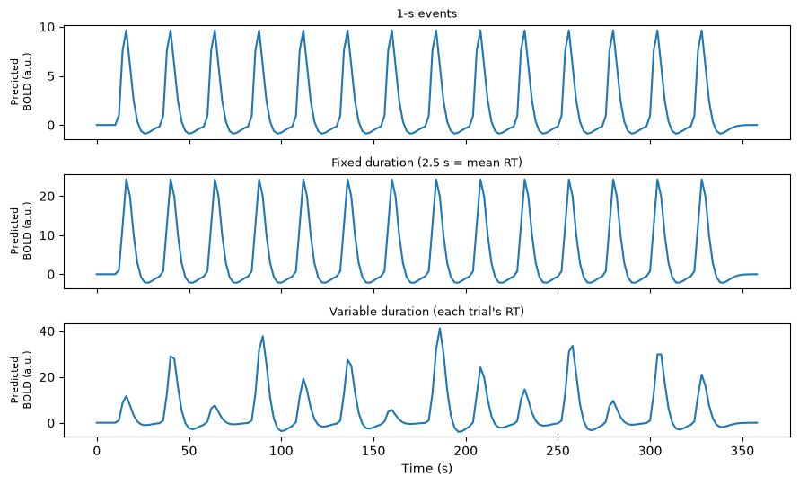
The three predictors share the same onsets but differ in shape and, for the variable-duration model, in trial-to-trial amplitude and width: long-RT trials produce larger, wider predicted responses. The fixed- and variable-duration regressors are highly correlated but not identical — the difference between them is exactly the RT-related information. Under linear-time-invariant assumptions, duration modulation and amplitude modulation are nearly indistinguishable for durations under ~1–2 s, and diverge as durations grow (long boxcars widen and plateau rather than just scaling up).
2. Parametric modulation
A parametric modulator asks a different question: does the response amplitude scale with a trial-by-trial variable — pain ratings, stimulus value, RT? The modulated regressor is entered alongside the unmodulated average-response regressor:
the average beta captures the response to a typical event
the modulator beta captures how the response scales with the variable
We build the modulator by weighting each trial’s stimulus impulse by its rating before convolving. Crucially, we compare a raw (uncentered) modulator with a mean-centered one.
ratings = np.array([3, 5, 2, 7, 4, 6, 1, 8, 5, 3, 7, 2, 6, 4.0])  # 1 per trial

x_avg = make_regressor(onsets, 1.0)                              # average response
xmod_raw      = make_regressor(onsets, 1.0, ratings)             # raw modulator
xmod_centered = make_regressor(onsets, 1.0, ratings - ratings.mean())

fig, axes = plt.subplots(2, 1, figsize=(9, 4.2), sharex=True)
axes[0].plot(frame_times, x_avg, lw=1.5, label="average response")
axes[0].plot(frame_times, xmod_raw, lw=1.5, ls="--", label="raw modulator")
axes[0].legend(fontsize=8); axes[0].set_title("Raw (uncentered) modulator", fontsize=9)
axes[1].plot(frame_times, x_avg, lw=1.5, label="average response")
axes[1].plot(frame_times, xmod_centered, lw=1.5, ls="--", label="centered modulator")
axes[1].legend(fontsize=8); axes[1].set_title("Mean-centered modulator", fontsize=9)
axes[1].set_xlabel("Time (s)")
plt.tight_layout()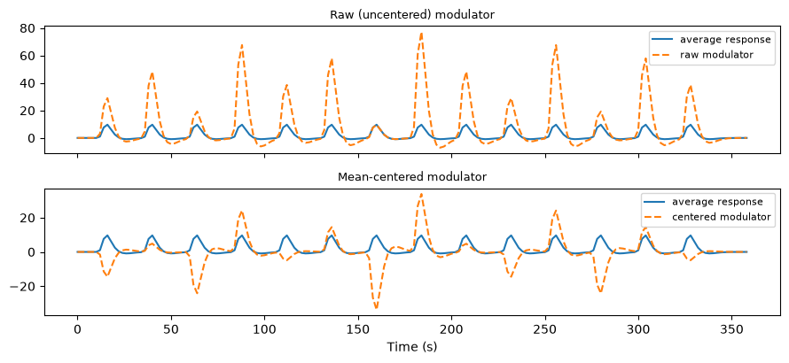
3. Collinearity: correlations and variance inflation factors
The modulator is built from the same onsets as its parent regressor, so the two are often substantially correlated. Pairwise correlations do not tell the whole story, though — what matters is whether one predictor can be written as a linear combination of all the others. The variance inflation factor captures this:
VIFᵢ — variance inflation factor for predictor i · Rᵢ² — proportion of variance in predictor i explained by all the other predictors
where is the variance inflation factor for predictor and is the coefficient of determination (proportion of variance explained) from regressing predictor on all the other predictors in the design matrix.
VIF = 1 is ideal; VIF = 2 means the variance of has doubled relative to an orthogonal design. In fMRI, VIFs above ~4 warrant serious attention, and above 8 power suffers dramatically and effects are easily misattributed.
def vifs(X, names=None):
    """VIF for each column of X (task/nuisance regressors, no constant).
    Computed from the inverse of the correlation matrix, as in getvif.m."""
    X = np.asarray(X, float)
    v = np.diag(np.linalg.inv(np.corrcoef(X, rowvar=False)))
    return pd.Series(v, index=names if names is not None
                     else [f"x{i}" for i in range(X.shape[1])])

r_raw = np.corrcoef(x_avg, xmod_raw)[0, 1]
r_cen = np.corrcoef(x_avg, xmod_centered)[0, 1]
print(f"corr(avg, raw modulator)      = {r_raw:.2f}")
print(f"corr(avg, centered modulator) = {r_cen:.2f}\n")

tab = pd.DataFrame({
    "VIF (raw)":      vifs(np.column_stack([x_avg, xmod_raw])).to_numpy(),
    "VIF (centered)": vifs(np.column_stack([x_avg, xmod_centered])).to_numpy(),
}, index=["Average", "Modulator"])
print(tab.round(2))
corr(avg, raw modulator) = 0.89
corr(avg, centered modulator) = -0.00
VIF (raw) VIF (centered)
Average 4.68 1.0
Modulator 4.68 1.0
Mean-centering is the essential first step, and it is what SPM and nilearn do by default. With evenly spaced onsets like these it removes essentially all of the collinearity (VIF → 1.0); with jittered or clustered onsets some usually remains. With the raw modulator, VIFs are already near 5: the average and modulated regressors carry nearly the same information, and neither beta can be estimated stably.
Cross-check with nilearn
make_first_level_design_matrix accepts a modulation column in the events table. Give the average-response rows a modulation of 1 and the modulator rows the centered ratings, and it reproduces our hand-built pair.
ev  = pd.DataFrame({"onset": onsets, "duration": 1.0,
                    "trial_type": "pain", "modulation": 1.0})   # average response
mod = ev.assign(trial_type="pain_x_rating",
                modulation=ratings - ratings.mean())            # mean-center!

X_nl = make_first_level_design_matrix(frame_times,
                                      pd.concat([ev, mod], ignore_index=True),
                                      hrf_model="spm", drift_model=None)

for ours, name in [(x_avg, "pain"), (xmod_centered, "pain_x_rating")]:
    r = np.corrcoef(ours, X_nl[name])[0, 1]
    print(f"hand-built vs. nilearn '{name}': r = {r:.3f}")
[make_first_level_design_matrix] A 'modulation' column was found in the given events data and is used.
hand-built vs. nilearn 'pain': r = 1.000
hand-built vs. nilearn 'pain_x_rating': r = 1.000
4. The orthogonalization experiment
It is tempting to “fix” a correlated pair by orthogonalizing one regressor with respect to the other. SPM does this automatically for parametric modulators. But orthogonalization does not create information — it reassigns the shared variance. Let’s prove it.
We simulate a voxel whose true response contains both an average effect () and a modulator effect (), then fit the pair two ways — as-is and with the modulator orthogonalized with respect to the average regressor — using both the raw (highly correlated) and the mean-centered modulator.
Watch which beta changes and which does not.
rng = np.random.default_rng(42)   # seed for reproducibility
n = n_scans                       # number of volumes (180)

# True voxel: average response (beta = 1.0) + rating-dependent scaling (beta = 0.5)
y = 100 + 1.0 * x_avg + 0.5 * xmod_centered + 2 * rng.standard_normal(n)

A = np.column_stack([x_avg, np.ones(n)])      # what we orthogonalize against

def orthogonalize(x):
    """Residuals of x after regressing out the average regressor + intercept."""
    return x - A @ np.linalg.lstsq(A, x, rcond=None)[0]

rows = {}
for label, xmod in [("raw modulator", xmod_raw),
                    ("centered modulator", xmod_centered)]:
    Xc = np.column_stack([x_avg, xmod,                np.ones(n)])   # as-is
    Xo = np.column_stack([x_avg, orthogonalize(xmod), np.ones(n)])   # orthogonalized
    b_c = np.linalg.lstsq(Xc, y, rcond=None)[0]
    b_o = np.linalg.lstsq(Xo, y, rcond=None)[0]
    rows[label] = [np.corrcoef(x_avg, xmod)[0, 1],
                   b_c[0], b_o[0], b_c[1], b_o[1]]

print(pd.DataFrame(rows, index=["corr(avg, modulator)",
                                "Average beta   -- as-is",
                                "Average beta   -- orthogonalized",
                                "Modulator beta -- as-is",
                                "Modulator beta -- orthogonalized"]).round(3))
print("\nTrue values: average = 1.0, modulator = 0.5")
raw modulator centered modulator
corr(avg, modulator) 0.887 -0.000
Average beta -- as-is -1.191 0.968
Average beta -- orthogonalized 0.968 0.968
Modulator beta -- as-is 0.480 0.480
Modulator beta -- orthogonalized 0.480 0.480
True values: average = 1.0, modulator = 0.5
The modulator’s beta is identical in both models — in the correlated model it already reflects the unique (partial) effect of the modulator, controlling for the average response. What changed is the average regressor’s beta. With the raw modulator the two regressors correlate at , and the as-is average beta is wildly off (even negative), because the raw modulator — whose mean rating is ~4.4 — is itself carrying the average response. Orthogonalizing hands that shared variance back to the average regressor and restores a sensible estimate. With the centered modulator the two regressors are already nearly orthogonal, so orthogonalization changes almost nothing: there was no shared variance to reassign.
Two lessons. First, mean-center your modulators — that fixes the real problem. Second, orthogonalization only decides who gets credit for shared variance. For a parametric modulator that is arguably right: the average regressor should get credit for the average response, and the modulator should capture only trial-to-trial scaling beyond it. But orthogonalizing an RT regressor with respect to condition regressors destroys its ability to control for RT confounds across conditions — the condition betas then still contain the RT-related variance. Orthogonalize only when you have a principled reason to assign the shared variance to one regressor.
5. High-pass filtering inside the GLM: the cosine drift set
fMRI signal drifts slowly even without a task (scanner instabilities, motion, aliased physiology), so most noise power lives at the lowest frequencies. Instead of pre-filtering the data (in which case the design matrix must be filtered identically!), we can add a discrete cosine transform (DCT) basis spanning all frequencies below the cutoff as columns of . For a cutoff period of 128 s (the SPM default, 0.0078 Hz):
def dct_basis(n, run_len_s, cutoff_s=128.0):
    """SPM-style DCT drift matrix: constant + cosines below 1/cutoff Hz."""
    k = int(2 * run_len_s / cutoff_s + 1)          # number of basis functions
    t = np.arange(n)
    C = np.ones((n, k)) / np.sqrt(n)
    for j in range(1, k):
        C[:, j] = np.sqrt(2 / n) * np.cos(np.pi * (2 * t + 1) * j / (2 * n))
    return C                                        # column 0 is the constant

drift = dct_basis(n_scans, run_len, 128)   # 128-s cutoff (SPM default)
print(f"Cosine drift set: {drift.shape[1]} columns "
      f"(1 constant + {drift.shape[1]-1} cosines)")

fig, ax = plt.subplots(figsize=(9, 2.8))
ax.plot(frame_times, drift[:, 1:], lw=1.5)
ax.set(xlabel="Time (s)", title="Cosine drift regressors (128-s cutoff)")
plt.tight_layout()

def fit_task(X, y):
    """OLS fit; return the task beta (column 0), its SE, t, and df_e."""
    b = np.linalg.lstsq(X, y, rcond=None)[0]
    r = y - X @ b
    dfe = len(y) - X.shape[1]
    s2 = r @ r / dfe
    se = np.sqrt(s2 * np.diag(np.linalg.pinv(X.T @ X)))
    return b[0], se[0], b[0] / se[0], dfe

# Two kinds of drift: one unrelated to the task, one that happens to share
# the task's low-frequency structure (the projection of x_avg onto drift space)
P_drift = drift @ np.linalg.pinv(drift)
low = P_drift @ x_avg - (P_drift @ x_avg).mean()

scenarios = {
    "drift unrelated to task":  4 * np.sin(2 * np.pi * np.arange(n) / n * 1.5)
                                + np.linspace(0, -5, n),
    "drift correlated w/ task": 5 * low / low.std(),
}

res = []
for name, drift_sig in scenarios.items():
    y2 = 100 + 1.0 * x_avg + drift_sig + 2 * rng.standard_normal(n)
    for model, X in [("no drift model", np.column_stack([x_avg, np.ones(n)])),
                     ("with drift set", np.column_stack([x_avg, drift]))]:
        res.append((name, model) + fit_task(X, y2))

print(pd.DataFrame(res, columns=["drift", "model", "beta (true 1.0)",
                                 "SE", "t", "df_e"]).round(3).to_string(index=False))
Cosine drift set: 6 columns (1 constant + 5 cosines)
drift model beta (true 1.0) SE t df_e
drift unrelated to task no drift model 1.024 0.079 12.969 178
drift unrelated to task with drift set 1.016 0.045 22.542 173
drift correlated w/ task no drift model 1.199 0.116 10.360 178
drift correlated w/ task with drift set 1.059 0.045 23.502 173
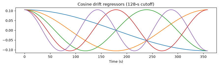
Two things happen when drift is left unmodeled. Always, the slow noise lands in the residuals: is inflated, the standard error roughly doubles, and the t-statistic is roughly halved — a big power loss for five degrees of freedom. And whenever the drift shares structure with the task (bottom rows), the task beta is also biased, because the unmodeled drift has nowhere to go but the task regressor. Adding the cosine set makes the accounting explicit: drift columns explain the drift, task columns explain the task.
What does the filter cost you? Check the contrast
Filtering is not free: any task variance below the cutoff is removed too. For block designs the rule of thumb is a cutoff period of roughly twice the task period. Event-related designs are trickier, because their variance is spread across frequencies — and what matters is the variance of the contrasts you care about, not just the individual regressors. Below we build randomized two-condition event-related designs and measure how much variance an 80-s filter removes from each regressor and from the A − B contrast.
rng2 = np.random.default_rng(3)   # separate seed for design randomization

def random_design():
    """28 jittered events, randomly labelled A or B."""
    ons = np.sort(rng2.uniform(8, run_len - 20, 28))
    lab = rng2.permutation(np.array(["A"] * 14 + ["B"] * 14))
    return make_regressor(ons[lab == "A"], 1.0), make_regressor(ons[lab == "B"], 1.0)

D = dct_basis(n_scans, run_len, cutoff_s=80)     # 80-s filter
P = D @ np.linalg.pinv(D)                        # projection onto drift space

def pct_var_removed(x):
    xf = x - P @ x                               # filtered regressor
    xc = x - x.mean()
    return 100 * (1 - (xf @ xf) / (xc @ xc))

# One design in detail, then the distribution over 200 random orderings
x_A, x_B = random_design()
for name, x in [("A", x_A), ("B", x_B), ("A - B contrast", x_A - x_B)]:
    print(f"this design -- variance removed from {name:16s}: {pct_var_removed(x):5.1f}%")

loss = np.array([[pct_var_removed(a), pct_var_removed(b), pct_var_removed(a - b)]
                 for a, b in (random_design() for _ in range(200))])

summary = pd.DataFrame(loss, columns=["A", "B", "A - B"]).describe(
    percentiles=[0.5, 0.9]).loc[["50%", "90%", "max"]].round(1)
print("\nOver 200 random orderings (% variance removed by the 80-s filter):")
print(summary)
print(f"orderings where the contrast loses more than either regressor: "
      f"{100 * np.mean(loss[:, 2] > loss[:, :2].max(axis=1)):.0f}%")

fig, ax = plt.subplots(figsize=(7, 3))
ax.hist(loss[:, 0], bins=25, alpha=0.55, label="regressor A")
ax.hist(loss[:, 2], bins=25, alpha=0.55, label="A - B contrast")
ax.set(xlabel="% variance removed by 80-s high-pass filter",
       ylabel="designs", title="Filter cost depends on the random ordering")
ax.legend(fontsize=8)
plt.tight_layout()
this design -- variance removed from A : 2.9%
this design -- variance removed from B : 6.0%
this design -- variance removed from A - B contrast : 4.8%
Over 200 random orderings (% variance removed by the 80-s filter):
A B A - B
50% 14.1 13.4 13.4
90% 23.6 22.4 23.2
max 32.8 31.9 32.9
orderings where the contrast loses more than either regressor: 21%
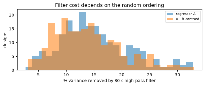
The first design we drew was a lucky one: the 80-s filter cost its contrast under 5% of its variance. Across 200 random orderings, though, the median contrast loss is ~13% — close to the ~12% in the book’s example — and the spread is wide, and in roughly one design in five the contrast loses more than either regressor does. That happens when the random ordering leaves slow stretches that are A-heavy or B-heavy, putting contrast energy below the cutoff. Filtering buys power only when it removes more noise than task-related signal, so check the cost on the contrasts you actually plan to test — before you collect data, when you can still re-randomize the design (Chapter 27).
6. Motion covariates, spike regressors, and task VIFs
Finally we assemble a realistic first-level design: task regressors plus nuisance covariates —
six realignment parameters (simulated here as slow random walks; real pipelines often expand them to 24 with squares and derivatives)
spike regressors: one indicator column per artifact-contaminated volume (flagged by framewise displacement, DVARS, or Mahalanobis distance). Spike regression absorbs all of a bad volume’s variance and is preferred to deleting volumes because it preserves the temporal structure needed for valid variances and P values
the cosine drift set from Section 5
Correlations among nuisance regressors are harmless — we never interpret their betas. What matters is nuisance–task correlation, which inflates the task VIFs. Comparing task VIFs with and without the nuisance set is a quick, powerful diagnostic you can run before ever touching brain data.
mot = np.cumsum(rng.standard_normal((n, 6)) * 0.02, axis=0)   # motion params

bad_vols = [40, 41]                                   # flagged volumes
spikes = np.zeros((n, len(bad_vols)))
for j, v in enumerate(bad_vols):
    spikes[v, j] = 1.0

X_task = np.column_stack([x_avg, xmod_centered])
X_full = np.column_stack([X_task, mot, spikes, drift[:, 1:]])  # + cosines
names_full = (["avg", "modulator"] + [f"mot{i+1}" for i in range(6)]
              + [f"spike{v}" for v in bad_vols]
              + [f"drift{i+1}" for i in range(drift.shape[1] - 1)])

v_alone = vifs(X_task, ["avg", "modulator"])
v_full  = vifs(X_full, names_full)
print(pd.DataFrame({"task alone": v_alone,
                    "full model": v_full[["avg", "modulator"]]}).round(2))

fig, ax = plt.subplots(figsize=(5, 5))
Z = (X_full - X_full.mean(0)) / X_full.std(0)
ax.imshow(Z, aspect="auto", cmap="gray", interpolation="nearest")
ax.set(xticks=range(len(names_full)), xlabel="", ylabel="Time (volumes)",
       title="Full first-level design: task, motion, spikes, drift")
ax.set_xticklabels(names_full, rotation=90, fontsize=7)
plt.tight_layout()
task alone full model
avg 1.0 1.04
modulator 1.0 1.13
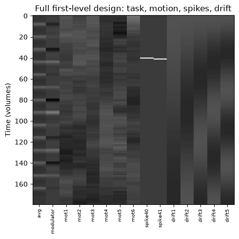
Here the task VIFs barely move: simulated motion and drift are (by construction) nearly unrelated to the task, so the nuisance set is cheap insurance. With real data, motion is often task-correlated (people move when they respond, swallow at block boundaries) — task VIFs then jump, and significance rightly drops, because task and artifact are genuinely confounded.
Every nuisance column also costs one error degree of freedom: with 180 volumes and this design we still have plenty, but with 24 motion covariates + CompCor + many spikes in a short run, can erode quickly. Less aggressive strategies with fewer regressors are often preferred.
Where to go next
Autocorrelated errors: the residuals of every model above are still autocorrelated — AR models, prewhitening, and generalized least squares make first-level P values valid
Chapter 20: contrasts and inference — coding and testing any comparison of conditions
Chapter 27: design efficiency — choosing onsets and orderings that keep VIFs low and contrast variance high before you scan
Exercises
Make one motion regressor task-correlated (
mot[:, 0] += 0.1 * x_avg) and re-run Section 6. What happens to the task VIFs? Simulate data and check what happens to the task betas’ standard errors.Halve the filter cutoff in Section 5 (64 s). How many drift columns are added, how many are lost, and how much more contrast variance is removed?
In Section 4, orthogonalize the average regressor with respect to the modulator instead. Which beta is unchanged now? Explain why in terms of shared-variance assignment.
Build a variable-duration RT regressor (Section 1) and an RT parametric modulator for the same trials, and compute the VIF of each with the average regressor in the model. Which representation is more separable from the average response, and why?