fMRI Basics and Terminology
Run this code: ⚡ In-browser lab · Colab · MATLAB Online
Overview
This chapter begins our journey into fMRI data analysis by establishing the vocabulary you will use for everything that follows. MR images are acquired within a field of view (FOV) — the volume of space in which data are collected, with the brain usually centered inside it. In echo planar imaging (EPI), data are acquired as a stack of two-dimensional slices, each sampled on a grid whose number of elements is the matrix size (e.g., 64 × 64). The FOV divided by the matrix size gives the in-plane resolution (e.g., 192 mm / 64 = 3 mm), and together with the slice thickness this determines the size of each voxel — a volumetric pixel, the elementary unit of an MR image. Larger voxels collect more signal relative to noise; smaller voxels resolve finer spatial detail. Many modern sequences acquire 3 × 3 × 3 mm isotropic voxels (equal size in all dimensions), close to an optimal balance at 3T.
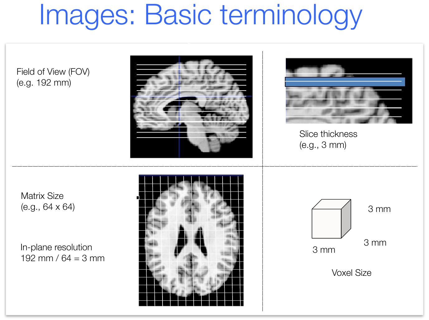
Basic MR image terminology. The field of view, slice thickness, matrix size, and in-plane resolution together determine the voxel size — and hence the spatial resolution of the image. (Figure 12.1 from the book. © the authors and MIT Press; reproduced with permission — not covered by this site’s CC-BY license.)
Once acquired, a 3-D volume can be displayed as slices in any orientation. Axial (horizontal) slices cut from bottom to top, coronal slices from front to back, sagittal slices from left to right, and oblique slices at other angles. Each dimension of brain space has a name and an axis: the left–right dimension is x, the posterior–anterior (back–front) dimension is y, and the inferior–superior (bottom–top) dimension is z. Anterior is also called rostral (“toward the head”) and posterior caudal (“toward the tail”); inferior locations are ventral (“toward the belly”) and superior ones dorsal (“toward the back”) — though in the brainstem, which lies parallel to the back, dorsal means toward the back of the head and rostral means toward the midbrain. Locations are reported as [x, y, z] coordinate triplets in millimeters relative to an origin at the anterior commissure, a small white-matter bundle connecting the hemispheres. Beware, though: conventions differ. SPM and FSL use the “LPI” convention (negative x = left), while AFNI’s default “RAI”/DICOM convention reverses the signs of x and y. This book uses LPI throughout.
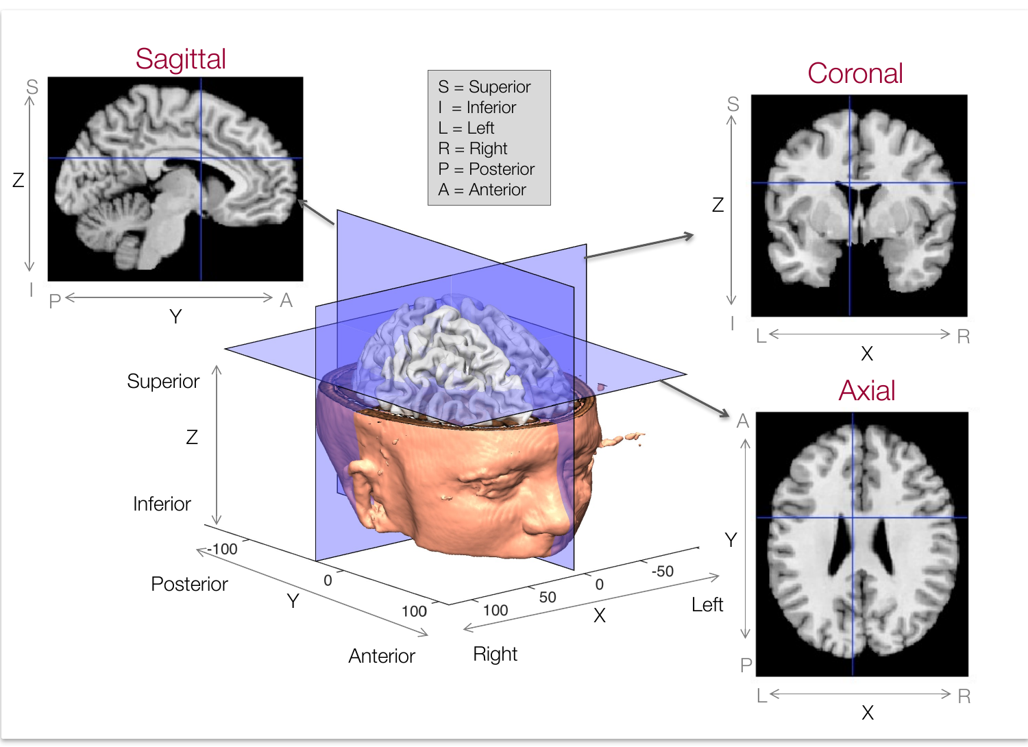
Nomenclature for standard coordinate space and anatomical position. The brain can be visualized in sagittal, coronal, or axial slices; x runs left–right, y posterior–anterior, and z inferior–superior. (Figure 12.2 from the book. © the authors and MIT Press; reproduced with permission — not covered by this site’s CC-BY license.)
An fMRI run is a time series of 3-D volumes acquired while the participant performs a task or rests. One volume is collected every repetition time (TR) — typically 2–3 seconds in older studies, and under 500 ms with modern accelerated (“multiband”) sequences. Functional (T2*-weighted) images have lower spatial resolution and less tissue contrast than structural (T1-weighted) images, but their signal fluctuations over time track local blood flow and oxygen metabolism, which in turn reflect neural activity. The absolute image values are arbitrary; what carries information is relative change across time, quantified for example as percentage signal change. Fixing one voxel’s position and extracting its intensity at every TR yields that voxel’s time series — the fundamental object of fMRI analysis. A single volume commonly contains 100,000 or more voxels, each with its own time series, making fMRI a “time series problem on steroids.”
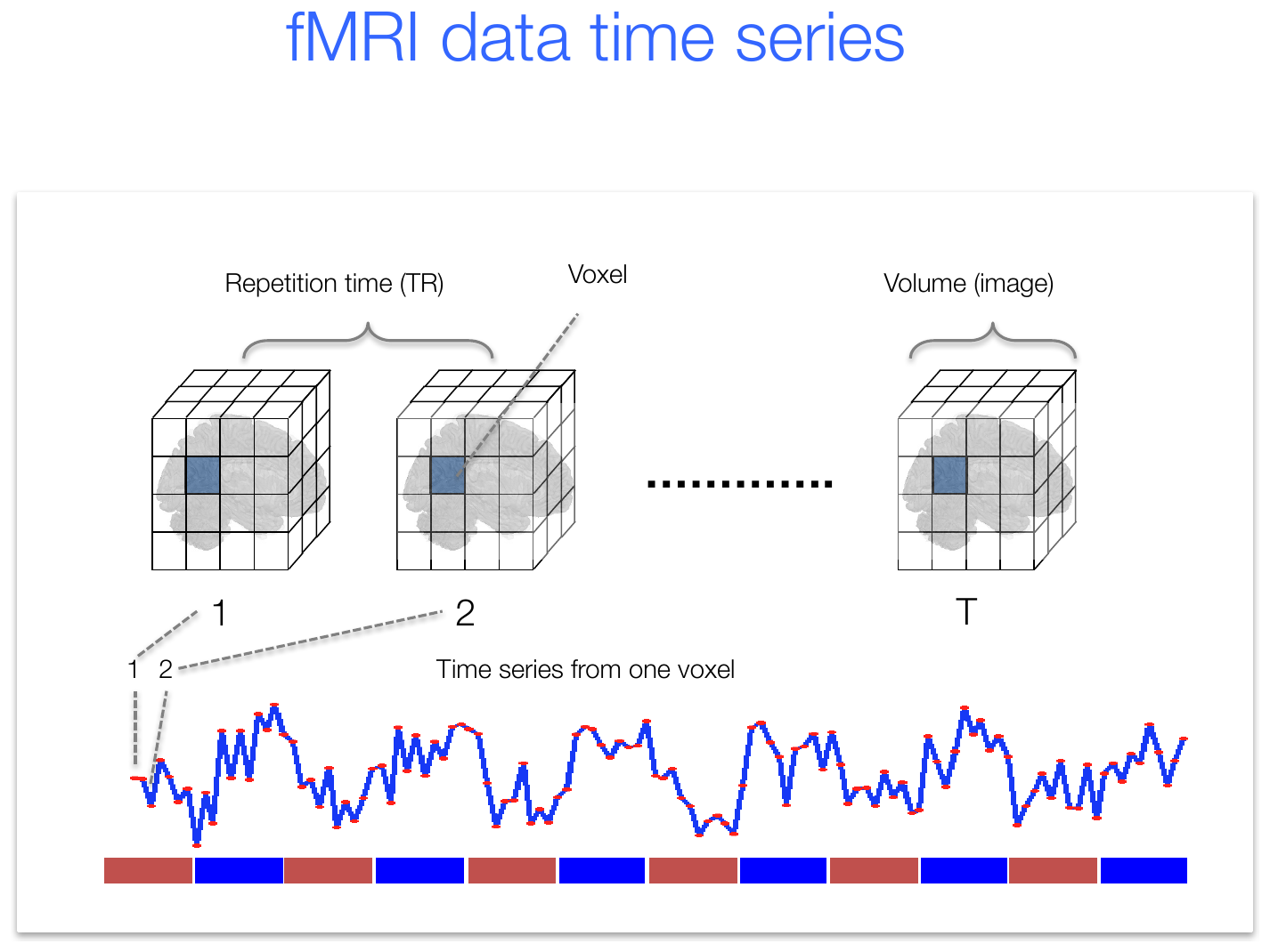
Terminology and sampling of fMRI time series. One brain volume is acquired every TR; fixing a voxel’s position and extracting its intensity at each TR yields a time series that can be related to an experimental task — here an on–off “block” (or “boxcar”) design shown as red and blue bars. (Figure 12.5 from the book. © the authors and MIT Press; reproduced with permission — not covered by this site’s CC-BY license.)
A standard analysis pipeline flows from experimental design through data acquisition and reconstruction into a series of preprocessing steps — slice-timing correction, motion correction, co-registration of functional to structural images, spatial normalization (warping) to a standard anatomical reference space, and often spatial smoothing and denoising — before statistical analysis. In task fMRI, voxels are typically analyzed one at a time (“mass-univariate” analysis), most often with multiple regression relating each voxel’s time series to the task design, while accounting for the slow, delayed hemodynamic response function (HRF) that peaks about 5–6 seconds after neural activity. Multivariate methods that model many voxels jointly are increasingly common as well.
The data themselves are fundamentally hierarchical: voxels are nested within slices, slices within volumes, volumes within runs (typically 4–10 minutes each), runs within scanning sessions, sessions within participants, and participants sometimes within groups. This structure shapes analysis: a first-level analysis models each participant’s time series data, producing contrast maps of experimental effects, which become input to a second-level analysis that tests reliability across participants and differences between groups or individuals.
Finally, images live in files with particular formats and conventions. Scanners produce DICOM files (one slice, one time point each — a study can generate millions); analysis packages convert these to NIfTI format (.nii), which stores a 3-D volume or a 4-D time series in a single file along with meta-data, including the affine matrix that maps voxel (matrix) coordinates to world (mm) coordinates. Writing a voxel’s indices as (its position in the data array) and its physical location as (in millimeters relative to the origin), the mapping is a single matrix–vector product in homogeneous coordinates:
[x, y, z] — world coordinates (mm, relative to the origin at the anterior commissure) · A — 4 × 4 affine matrix stored in the NIfTI header · [i, j, k] — voxel (matrix) indices into the data array · trailing 1 — homogeneous coordinate that lets A encode translations as well as scaling and rotation
where are voxel (matrix) indices into the data array, is the 4 × 4 affine matrix stored in the image header — its diagonal holds the voxel sizes in mm, its last column the origin, and off-diagonal entries any rotations — and are world coordinates in millimeters relative to the origin at the anterior commissure.
A notorious pitfall is left–right flipping: in radiological display format the brain’s left is on the image’s right (as if viewing the patient from the feet), whereas in neurological format — the standard in cognitive neuroscience — the brain’s right is on the image’s right. Because packages handle orientation meta-data differently, flipping errors appear even in published papers. Safeguards include consistent use of NIfTI and one software package, fiducial markers (a Vitamin E capsule taped to one side of the head), and anatomical heuristics — in most people the left occipital lobe is larger, pushing the calcarine fissure rightward (“left looms larger”). The cortex can also be analyzed on extracted 2-D surfaces (GIFTI and CIFTI “grayordinate” formats popularized by FreeSurfer and the Human Connectome Project). Most researchers work within a rich ecosystem of free packages — SPM, FSL, AFNI, FreeSurfer, and Python tools such as nilearn and Nipype, plus MATLAB toolboxes including the CANlab object-oriented tools — which can be combined, with care, into custom workflows.
Hands-on tutorial
In this tutorial you will build (Python) or load (MATLAB) a small 4-D dataset and connect the chapter’s vocabulary to real data structures: dimensions, voxel size, the affine voxel-to-world mapping, one voxel’s time series, and a slice montage.
Step 1 — Create or load a 4-D dataset and inspect its geometry. The header’s dimensions, zooms (voxel sizes and TR), and affine matrix encode everything about where the data sit in space and time.
% Requires CanlabCore + SPM12 on your MATLAB path
% Adapted from CANlab tutorials (github.com/canlab)
imgs = load_image_set('emotionreg', 'noverbose');  % 30 images in an fmri_data object

size(imgs.dat)               % .dat is a [voxels x images] data matrix
imgs.volInfo.dim             % image dimensions in voxels (x, y, z)
imgs.volInfo.mat             % affine: voxel (matrix) space -> world (mm) space

% Convert a voxel coordinate to world (mm) coordinates:
vox = [25 30 16 1]';         % [i j k 1]', homogeneous coordinates
mm  = imgs.volInfo.mat * vox % [x y z 1]' in mm relative to the origin
import numpy as np, nibabel as nib
from nibabel.affines import apply_affine
rng = np.random.default_rng(0) # fixed seed, so results reproduce exactly
shape = (20, 24, 12, 60) # (x, y, z, t): 20 x 24 matrix, 12 slices, 60 volumes
data = 100 + rng.standard_normal(shape) # baseline ~100 a.u. + noise (absolute values are arbitrary)
affine = np.diag([3.0, 3.0, 3.0, 1.0]) # 3 mm isotropic voxels
affine[:3, 3] = [-28.5, -34.5, -16.5] # so world (0,0,0) is mid-volume
img = nib.Nifti1Image(data, affine)
img.header.set_zooms((3.0, 3.0, 3.0, 2.0)) # 4th zoom = TR in seconds
print(img.shape, img.header.get_zooms())
print(apply_affine(affine, [9, 11, 5])) # voxel [i, j, k] -> mmExample output:
(20, 24, 12, 60) (np.float32(3.0), np.float32(3.0), np.float32(3.0), np.float32(2.0))
[-1.5 -1.5 -1.5]
The image is 20 × 24 × 12 voxels × 60 volumes, with 3 mm voxel sizes and the 2-s TR stored as the header “zooms.” Voxel [9, 11, 5] maps to [−1.5, −1.5, −1.5] mm — just off the world origin, because the exact volume center falls between voxels.
Step 2 — Extract one voxel’s values and view slices. A voxel’s time series is the raw material of every analysis to come; a montage of slices is the standard way to view a whole volume at once.
m = mean(imgs);                       % mean image across the 30 images
orthviews(m);                         % interactive 3-view (orthogonal) display
figure; axis off; montage(m);         % canonical slice montage

% One voxel's values across the columns of .dat:
v = imgs.dat(1000, :)';               % row 1000 = one voxel; columns = the 30 images
figure; plot(v, 'o-');
xlabel('Image number'); ylabel('Value (a.u.)');
import matplotlib.pyplot as plt
ts = data[9, 11, 5, :] # one voxel's time series: fix [i, j, k], keep all TRs
t = np.arange(shape[3]) * 2.0 # time axis in seconds: volume number x TR (2 s)
fig, ax = plt.subplots(figsize=(7, 2.5))
ax.plot(t, ts); ax.set(xlabel='Time (s)', ylabel='Signal (a.u.)')
mean_vol = data.mean(axis=3) # average volume over time
fig, axes = plt.subplots(2, 6, figsize=(9, 3)) # 12 axial slices in a 2 x 6 grid
for k, ax in enumerate(axes.ravel()): # one axial slice per panel
ax.imshow(mean_vol[:, :, k].T, cmap='gray', origin='lower')
ax.axis('off')Example output:
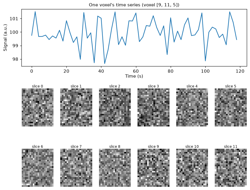
Output of the Python tab: one voxel’s time series (top) and the axial slice montage of the mean volume (bottom). These simulated volumes are pure noise around a baseline of 100, so the slices look like static — in the full lab you build a brain-shaped dataset with an “active” region and watch it emerge from exactly these views.
The full labs go further: simulating an “active” region with a boxcar task signal, saving and reloading NIfTI files, converting between voxel and world coordinates in both directions, and displaying the same slice in radiological and neurological orientation.
Open the full Python lab notebook → or download the MATLAB live script, which mirrors it using CANlab tools.


Thought questions
You are designing two studies: one mapping fine-grained activity patterns in the brainstem, the other tracking rapid signal changes during a fast event-related task. For each, how would you weigh voxel size, TR, FOV coverage, and signal-to-noise against one another, and why do these choices trade off at all?
A collaborator sends you activation coordinates from a paper analyzed in AFNI using its default coordinate convention, and you plot them on your LPI-convention template. What specific errors could result, how might they go unnoticed given the brain’s near-symmetry, and what checks would you build into your workflow to catch them?
fMRI data are hierarchical: volumes within runs, runs within sessions, sessions within participants, participants within groups. Why do researchers typically break long tasks into several short runs rather than one continuous scan, and how does the first-level/second-level analysis split reflect the hierarchy rather than being a mere computational convenience?
The absolute intensity values in fMRI images are arbitrary. What kinds of scientific questions does this render unanswerable with standard BOLD fMRI, and how do task-based and resting-state analyses each work around this limitation?
Combining tools across software packages (e.g., preprocessing in one package, statistics in another) is powerful but risky. Drawing on what you know about image headers, affine matrices, and orientation conventions, describe two concrete failure modes and how you would guard against each.
Quiz yourself
Q1. What is a voxel, and which two acquisition parameters jointly determine its size?
Answer: A voxel (“volumetric pixel”) is the small cubic volume within which the MR signal is sampled. Its size is set by the in-plane resolution (FOV divided by matrix size) and the slice thickness.
Q2. Name the three cardinal slice orientations and the direction each one cuts through the brain.
Answer: Axial (horizontal) slices cut at one location from bottom to top, coronal slices from front to back, and sagittal slices from left to right. Slices at other angles are called oblique.
Q3. What is the TR, and what are typical values in older versus modern accelerated acquisitions?
Answer: The TR (repetition time) is the time between successive whole-brain volumes. Typical TRs were 2–3 seconds in the early 2000s; with accelerated (multiband/simultaneous multi-slice) imaging, TRs under 500 ms are now common.
Q4. In the LPI convention used in this book, what do the x, y, and z axes represent, and where is the [0, 0, 0] origin?
Answer: x runs left to right, y posterior (back) to anterior (front), and z inferior (bottom) to superior (top). The origin is at the anterior commissure, a small white-matter bundle connecting the two hemispheres (though in the MNI152 template the marked zero-point sits slightly dorsal and posterior to it).
Q5. What is the difference between radiological and neurological display formats?
Answer: In radiological format the brain’s left side appears on the right of the displayed image, as if looking up at the person from their feet. In neurological format — standard in cognitive neuroscience — the brain’s right side appears on the right of the image.
Q6. How do DICOM and NIfTI files differ in what they store, and what does a 4-D NIfTI file contain?
Answer: A DICOM file holds a single slice at a single time point plus extensive header meta-data, so one study can comprise millions of files. NIfTI (.nii) is a standard format storing a whole 3-D volume — or, in 4-D form, an entire time series of volumes (e.g., one participant’s run) — in a single file with its spatial meta-data.
Q7. What is the difference between a first-level and a second-level analysis?
Answer: A first-level analysis models each individual participant’s voxel time series (typically mass-univariate regression), producing contrast maps of experimental effect magnitudes. A second-level analysis takes those contrast maps as input and tests effect reliability across participants, including group differences and individual-difference effects.
Q8. What does “mass-univariate” analysis mean, and how does it differ from multivariate analysis?
Answer: Mass-univariate analysis fits a separate statistical model to each voxel’s time series independently and assembles the results into a statistical map. Multivariate analyses instead model many voxels simultaneously — they are multivariate in brain space — for example to decode or predict experimental conditions from distributed activity patterns.
 The book: Elements of Functional Magnetic Resonance Imaging — Wager & Lindquist, MIT Press