Experimental Design and Task fMRI
Run this code: ⚡ In-browser lab · Colab · MATLAB Online
Overview
Not all fMRI designs with the same trials are equal: the spacing and ordering of events is critical. A good task fMRI design seeks to do three things: (1) manipulate the specific psychological processes to be mapped onto brain activity; (2) detect brain responses to those events with maximal sensitivity and specificity; and (3) maximize the internal and external validity of the resulting inferences. The experimenter’s levers are which stimuli to present and when to present them — and those timing choices have both psychological and statistical consequences.
The most basic choice is how to organize events in time. Block designs group events of one type into extended intervals (e.g., 16–20 s of condition A, then condition B), driving sustained responses that alternate slowly. Event-related designs randomize the order and timing of brief individual events, allowing responses to specific event types to be isolated. Dense event-related designs pack events with little rest; sparse designs include more rest and typically “jitter” the inter-trial interval. Hybrid (mixed) designs intermix both levels — block regressors capture sustained, state-like processes (e.g., goal maintenance during high-conflict blocks), while event regressors capture stimulus-evoked responses within blocks. Broadly, block designs provide high power to detect activation differences but imprecise information about which brief psychological events drive them; event-related designs link activity to specific events more precisely, with better control over predictability and trial history, but usually at a cost in power.
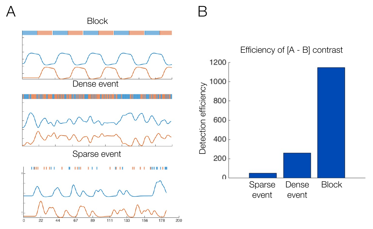
Arranging trials in a simple task fMRI design. (A) Block designs alternate sustained blocks of each condition; dense event-related designs intermix events with little rest; sparse event-related designs add jittered rest periods. Events for conditions A (blue) and B (red) are shown above their corresponding regressors. (B) Detection efficiency for an A − B contrast: block designs induce the most contrast variance and are most efficient; sparse event-related designs are least efficient. (Figure 27.1 from the book. © the authors and MIT Press; reproduced with permission — not covered by this site’s CC-BY license.)
Timing choices are psychological as well as statistical. The analysis assumes the process of interest is engaged at specific, known times — but participants may ruminate or shift attention during long rests, experience unplanned processes (frustration on “easy” trials, conflict carried over from trial history), or adopt unintended strategies (verbally labeling stimuli in a “spatial” task). Such deviations cost power and can create outright confounds. A good task incentivizes and constrains performance, maximizes time on task and the size of the induced effect, measures whether participants actually did the task, and anticipates side effects such as anticipation, habituation, learning, fatigue, and boredom.
The statistical quality of a design is captured by its efficiency: the ability to estimate task effects with low variance, which translates directly into statistical power. Recall that the t-statistic for a parameter divides the estimate by its standard error, and that the standard error factors into a noise term and a term that depends purely on the design matrix:
t — t-statistic for parameter i · β̂ᵢ — estimated parameter · SE — standard error · σ̂² — estimated residual noise variance · X — design matrix (time × predictors) · [(XᵀX)⁻¹]ᵢᵢ — i-th diagonal element: the design-related variance component
where is the estimated parameter for regressor , the estimated residual noise variance, the design matrix (time points × predictors), and the -th diagonal element of — the component of the variance determined purely by the design.
Because the design term is known before any data are collected, we can score candidate designs in advance. Averaging the design-related variance across the regressors and inverting gives the efficiency, known as A-optimality in the experimental design literature:
e — average design efficiency (A-optimality) · p — number of regressors · trace — sum of the diagonal elements · e_c — efficiency of a specific contrast · c — contrast vector (e.g., [1 −1 0] for A − B) · X — design matrix
where is the efficiency averaged over the regressors, the sum of the diagonal elements, the efficiency of a specific contrast, and the contrast vector.
The second form scores a specific contrast vector (e.g., for A − B). Efficiency is maximized when there are many observations, when predictor variance is high (predicted signal swings between extremes rather than hovering near its mean), and when regressors are close to orthogonal. High diagonal elements of mean imprecise parameter estimates; high off-diagonal elements mean confusable parameter estimates, so that true signal for one regressor can masquerade as activation or deactivation for another.
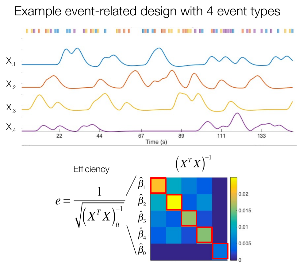
Efficiency in a four-condition event-related design. Top: regressors – for the four event types. Bottom: the matrix determines the design-related component of the standard errors — higher diagonal values (red boxes) mean higher standard errors and reduced power, and off-diagonal values mean correlated, confusable parameter estimates. (Figure 27.2 from the book. © the authors and MIT Press; reproduced with permission — not covered by this site’s CC-BY license.)
Two refinements shape practical design choices. First, nonlinearity: the BOLD response is roughly linear when events are at least 5 s apart, but responses to stimuli within 1–2 s of a preceding stimulus are substantially reduced and delayed — vascular saturation that the standard linear model ignores. Rapid designs are therefore dramatically less efficient in practice than the linear model predicts, and nonlinear history effects can confound condition comparisons unless trial history is equated across conditions. Second, jitter: with variable ISIs, runs of same-type trials let predicted activity build to peaks and fall to valleys, creating the variance needed to compare events to an implicit resting baseline. If the only goal is comparing event types (A − B), randomizing order achieves good rise and fall without extra jitter; but jitter is critical for asking whether events activate or deactivate a region relative to baseline. A popular recipe is jittered ISIs of at least 4 s with exponentially decreasing frequencies of longer delays up to ~16 s.
A closely related diagnostic is the variance inflation factor (VIF). Pairwise correlations miss the real danger — a regressor that is predictable from a combination of the others — so for each regressor we regress it on all remaining regressors and compute
VIFⱼ — variance inflation factor for regressor j · Rⱼ² — variance in regressor j explained by all the other regressors together
where is the proportion of variance in regressor explained by regressing it on all the other regressors.
is the multiplicative increase in that parameter’s variance due to the other regressors. A VIF of 1 is perfect (orthogonal); values above ~2 deserve attention, and values of 4–8+ signal serious trouble. In a designed experiment VIFs should be low — that is precisely the advantage of experiments over observational designs. Even when individual regressors are poorly estimable (e.g., two conditions with no rest between them), specific contrasts such as A − B may still be estimated precisely.
Beyond the block/event choice, several higher-level design types serve different inferential goals: subtraction designs compare conditions matched on all but the process of interest; parametric variation designs test whether activity tracks graded manipulations or measured variables (difficulty, reaction time, prediction error); and factorial designs cross factors to test main effects and interactions, supporting process association and dissociation. Eight principles summarize the practical tradeoffs: sample size (more subjects always helps, and group power is ultimately limited by , where is the number of participants, no matter how efficient the first level is); scan time per subject (30–40 min of functional data is a reasonable target, then spend the budget on subjects); number of conditions (fewer is more powerful, two is optimal for detection); grouping (blocks for detection, events for specific inference); block frequency (16–20 s blocks — longer blocks collide with high-pass filters, which then remove design variance); randomization (randomize per participant to avoid order confounds); nonlinearity (space events by several seconds, stratify randomization); and optimization.
That last principle can be automated. Programs like OptSeq evaluate huge numbers of random designs and keep the best, but the design space vastly exceeds brute-force search. Genetic algorithms (GAs) evaluate a population of designs, then recombine pieces of the best designs into “children” across generations — stochastic jumps in the fitness landscape that escape local maxima. A GA can weight multiple goals: which contrasts matter, a desired high-pass filter, counterbalancing, and whether to prioritize detection efficiency (precise contrast estimates given an assumed canonical HRF) or estimation efficiency (precise estimation of the HRF’s shape using a flexible FIR model). These two forms of efficiency strongly trade off: the alternating 16–18 s block design is optimal for detection but poor for shape estimation, m-sequences (pseudorandom sequences orthogonal to time-shifted copies of themselves) are optimal for estimation but poor for detection, and random event-related designs are mediocre at both. GA-optimized designs beat random designs on both criteria and approach the theoretical limit.
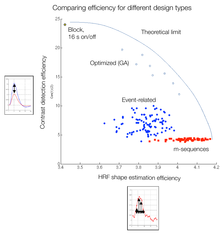
Design types compared on contrast detection and HRF shape estimation efficiency. The 16 s on/off block design (top left) is best for detection but poor for shape estimation; m-sequences (bottom right) are the reverse. Random event-related designs (blue) are intermediate on both, and GA-optimized designs (open circles) approach the theoretical limit (curve). (Figure 27.4 from the book. © the authors and MIT Press; reproduced with permission — not covered by this site’s CC-BY license.)
Efficiency calculations are powerful precisely because they require no data — you can score and optimize a design before ever entering the scanner. But they do not protect against unmodeled confounds or a mis-specified model (assuming linearity where there is none, or the wrong HRF), so those must be addressed on their own terms.
Hands-on tutorial
In this tutorial you will score competing designs before collecting any data: build a blocked, a dense fixed-ISI event-related, and a sparse jittered event-related design for two conditions, compute the efficiency of the A − B contrast for each, and diagnose collinearity with VIFs. The full labs extend this to the detection-versus-estimation tradeoff.
Step 1 — Build three competing designs and score the A − B contrast. Each design has two event types, A and B, in runs of equal length; only the arrangement in time differs.
% Requires CanlabCore + SPM12 on your MATLAB path
% Adapted from CANlab tutorials (github.com/canlab)
TR = 1;             % repetition time (s)
scanLength = 480;   % run length (s)
HP = 128;           % high-pass filter cutoff (s)
c = [1 -1 0];       % contrast: A minus B (last column = intercept)

% Blocked: 2 conditions, 16-s blocks, alternating
[Xb, eb] = create_block_design(scanLength, TR, 2, 16, HP, 0);

% Dense event-related: one 2-s event every 4 s, no rest (50/50 A/B)
[Xd, ed] = create_random_er_design(TR, 4, 2, [.5 .5], HP, 0, ...
                                   'scanLength', scanLength);

% Sparse jittered ER: same, but 50% of slots are rest (jitter)
[Xs, es] = create_random_er_design(TR, 4, 2, [.25 .25], HP, 0, ...
                                   'scanLength', scanLength);

% Efficiency of the A - B contrast: e = 1 / (c (X'X)^-1 c')
eff = @(X) 1 ./ (c * pinv(X) * pinv(X)' * c');
fprintf('A-B efficiency: block %3.1f, dense ER %3.1f, sparse ER %3.1f\n', ...
    eff(Xb), eff(Xd), eff(Xs));
import numpy as np
from scipy import stats
rng = np.random.default_rng(27) # seeded RNG so event orderings are reproducible
T, dt = 480, 1.0 # T = run length (s); dt = sampling step (s)
t = np.arange(0, T, dt) # time grid for the run
hrf = stats.gamma.pdf(t[:32], 6) - stats.gamma.pdf(t[:32], 16) / 6 # double-gamma HRF, 32-s window
def design(onsets_A, onsets_B, dur=2.0):
X = np.ones((len(t), 3)) # columns: A, B, intercept
for j, onsets in enumerate([onsets_A, onsets_B]):
s = np.zeros_like(t)
for on in onsets: s[(t >= on) & (t < on + dur)] = 1.0
X[:, j] = np.convolve(s, hrf)[:len(t)]
return X
# Blocked (16 s A / 16 s B), dense fixed-ISI ER, sparse jittered ER
X_block = design(np.arange(0, T, 32), np.arange(16, T, 32), dur=16)
lab = rng.permutation(np.repeat([0, 1], 60)) # 120 events, ISI 4 s
X_dense = design(np.arange(0, T, 4)[lab == 0], np.arange(0, T, 4)[lab == 1])
keep = rng.random(120) < 0.5 # 50% rest slots
X_sparse = design(np.arange(0, T, 4)[(lab == 0) & keep],
np.arange(0, T, 4)[(lab == 1) & keep])
c = np.array([1., -1., 0.]) # contrast: A minus B (last column = intercept)
eff = lambda X: 1.0 / (c @ np.linalg.pinv(X.T @ X) @ c) # e_c = 1 / (c (X'X)^-1 c')
for name, X in [("block", X_block), ("dense ER", X_dense), ("sparse ER", X_sparse)]:
print(f"{name:9s} e(A-B) = {eff(X):5.1f}")Example output:
block     e(A-B) =  87.8
dense ER  e(A-B) =  13.8
sparse ER e(A-B) =   6.7
The block design should win by a wide margin for the A − B contrast, with the sparse jittered design least efficient — exactly the ordering in Figure 27.1B. (The jittered design earns its keep elsewhere: comparing events to baseline and estimating HRF shape.)
Step 2 — Diagnose collinearity with variance inflation factors. Efficiency drops when regressors are correlated, and the danger is not always visible in pairwise correlations. We compute VIFs for the three designs above, then build the most common collinearity trap in real tasks: a cue event always followed by a stimulus event at a fixed short lag.
% VIFs (CanlabCore getvif): 1 = orthogonal; ~2+ warrants attention; 4-8+ trouble
designs = {Xb, Xd, Xs};  names = {'block' 'dense ER' 'sparse ER'};
for i = 1:3
    v = getvif(designs{i});                  % one VIF per task regressor
    fprintf('%-9s VIF(A) = %5.2f\n', names{i}, v(1));
end

% The classic task-programming trap: stimulus always 2 s after its cue
[~, ~, ons] = create_random_er_design(TR, 4, 2, [.25 .25], HP, 0, ...
                                      'scanLength', scanLength);
cue = ons{1}(:, 1);                    % cue onsets (s) from the sparse design
dur = 2 * ones(size(cue));             % 2-s event durations
lags = [2 6 10];                       % candidate cue->stimulus lags (s)
lag = lags(randi(3, numel(cue), 1))';  % one random lag per trial (jitter)

Xfix = onsets2fmridesign({[cue dur] [cue + 2   dur]}, TR, scanLength);
Xjit = onsets2fmridesign({[cue dur] [cue + lag dur]}, TR, scanLength);

vf = getvif(Xfix);  vj = getvif(Xjit);
fprintf('cue-stim, fixed 2-s lag: VIF %4.2f, e(A-B) %5.1f\n', vf(1), eff(Xfix));
fprintf('cue-stim, jittered lag : VIF %4.2f, e(A-B) %5.1f\n', vj(1), eff(Xjit));
def vif(X):
"""VIF for each non-intercept column of X: 1 / (1 - R_j^2)."""
Xc = X[:, :-1] - X[:, :-1].mean(axis=0) # drop intercept, center
out = []
for j in range(Xc.shape[1]):
yj, Xo = Xc[:, j], np.delete(Xc, j, axis=1)
b, *_ = np.linalg.lstsq(Xo, yj, rcond=None)
out.append(np.sum(yj**2) / np.sum((yj - Xo @ b)**2))
return np.array(out)
for name, X in [("block", X_block), ("dense ER", X_dense), ("sparse ER", X_sparse)]:
print(f"{name:9s} corr(A,B) = {np.corrcoef(X[:,0], X[:,1])[0,1]:5.2f}"
f" VIF(A) = {vif(X)[0]:6.2f}")
# The classic task-programming trap: stimulus always 2 s after its cue
cue = np.arange(0, T, 4)[(lab == 0) & keep] # cue onsets: the sparse design's A events
X_fixed = design(cue, cue + 2.0) # stimulus always 2 s after its cue
X_jit = design(cue, cue + rng.choice([2., 6., 10.], size=len(cue))) # jittered 2/6/10-s lag
for name, X in [("fixed 2-s lag", X_fixed), ("jittered lag ", X_jit)]:
print(f"cue-stim, {name}: VIF = {vif(X)[0]:5.2f} e(A-B) = {eff(X):5.1f}")Example output:
block     corr(A,B) = -0.98   VIF(A) =  29.55
dense ER  corr(A,B) = -0.98   VIF(A) =  20.61
sparse ER corr(A,B) = -0.30   VIF(A) =   1.10
cue-stim, fixed 2-s lag: VIF =  2.87   e(A-B) =   1.0
cue-stim, jittered lag : VIF =  1.01   e(A-B) =   4.0
Two lessons come out of this. First, the no-rest trap: the block and dense designs have enormous VIFs (roughly 20–30 here), because with an event always on, each regressor is nearly perfectly predictable from the other plus the intercept. No individual — “does A activate this region relative to rest?” — is well estimated, which is exactly why those designs are poor for baseline comparisons. Yet the A − B contrast is still estimated precisely: VIF is a per-parameter diagnostic, and a specific contrast can be precise even when its constituent parameters are not. The sparse jittered design keeps VIFs near 1.
Second, the fixed-lag trap: when a stimulus always follows its cue at the same short lag, the two convolved regressors correlate around 0.8, the VIF climbs past the warning zone, and the efficiency of the A − B contrast collapses several-fold — true cue-related signal can masquerade as stimulus activation, or deactivation. Jittering the cue-to-stimulus interval decorrelates the regressors and restores efficiency. Jitter is the cure.
The full labs go on to map the detection-versus-estimation tradeoff of Figure 27.4 by scoring many random designs under both a canonical-HRF model and an FIR model.
Open the full Python lab notebook → or download the MATLAB live script, which mirrors it using CANlab design tools (create_block_design, create_random_er_design, getvif, and the OptimizeDesign genetic algorithm).


Thought questions
Block designs are the most efficient way to detect an A − B difference, yet many cognitive neuroscientists avoid them. Considering psychological validity, predictability, trial-history effects, and the interpretability of the A − B contrast, when would you accept the efficiency loss of an event-related design — and when would that be a mistake?
Efficiency can be computed before any data are collected, and design optimizers maximize it aggressively. What can a highly “optimal” design still get wrong? Discuss at least three failure modes (e.g., HRF mis-specification, BOLD nonlinearity, psychological side effects of the optimized event sequence) and how you would guard against each.
A colleague proposes a rapid event-related design with a fixed 1.5-s ISI to “maximize the number of trials.” Using the concepts of nonlinearity, predictor variance, and collinearity with the intercept/baseline, explain what will happen to their ability to (a) contrast conditions A and B and (b) estimate activation relative to baseline.
Group-level power depends on both within-subject efficiency and between-subject variance. Given a fixed budget of scanner hours, how would you decide between scanning more participants briefly versus fewer participants longer? What property of your task and population would most change your answer?
The detection–estimation tradeoff implies no single design is best for everything. Design a study of a slow, uncertain process (e.g., pain anticipation) where you genuinely need both good HRF shape estimates and good contrast detection. What compromises would you make, and how could a genetic algorithm’s weighted fitness function encode them?
Quiz yourself
Q1. What distinguishes a block design from an event-related design, and what is a hybrid (mixed) design?
Answer: A block design groups events of one condition into extended intervals (e.g., 16–20 s) that alternate with other conditions; an event-related design randomizes the order and timing of brief individual events. Hybrid designs include both block-level regressors (sustained, state-like processes) and event-level regressors (stimulus-evoked responses) in the same experiment.
Q2. What is design efficiency, and why can it be computed before collecting any data?
Answer: Efficiency is the inverse of the design-related component of the parameter (or contrast) variance — e.g., for a contrast . Because the standard error factors into a noise term () and a term that depends only on the design matrix , the design term can be evaluated from the planned event timing alone, before any scanning.
Q3. Name the three main conditions under which efficiency is maximized.
Answer: (1) Many observations (more rows of , i.e., longer scans); (2) high predictor variance (predicted responses swing between extreme high and low values); and (3) low covariance/multicollinearity among regressors — ideally orthogonal predictors.
Q4. Why is jitter (variable ISI) essential if you want to compare event responses to baseline?
Answer: With jitter, runs of closely spaced same-type trials sum to high peaks while long gaps let the signal fall back toward baseline, creating condition-specific peaks and valleys. Without this variance relative to rest, event regressors are nearly constant and confounded with the intercept, so activation versus an implicit resting baseline cannot be estimated — though a difference contrast like A − B may still be fine.
Q5. What is a variance inflation factor, and roughly what values signal trouble?
Answer: , where comes from regressing predictor on all other predictors; it is the multiplicative increase in that parameter’s variance due to collinearity. A VIF of 1 means the regressor is orthogonal to the rest; values around 2+ warrant attention and values of roughly 4–8 or more indicate serious collinearity.
Q6. Over what event spacing is the BOLD response approximately linear, and what happens in rapid sequences?
Answer: Responses are roughly linear when events are at least ~5 s apart (with residual nonlinearity of about 10% even then). For stimuli within ~1–2 s of preceding stimuli, responses are substantially reduced in amplitude and delayed — vascular saturation — so rapid designs lose power in practice and history effects can confound condition comparisons.
Q7. What is the difference between detection efficiency and estimation efficiency, and how do they relate?
Answer: Detection efficiency is the precision of estimating condition effects or contrasts assuming a known (canonical) HRF; estimation efficiency is the precision of estimating the HRF’s shape itself using a flexible model such as FIR. The same efficiency formula applies with different design matrices, and the two strongly trade off: block designs maximize detection but are poor for shape estimation, while m-sequences do the reverse.
Q8. How does a genetic algorithm search for optimized fMRI designs, and why does it outperform purely random search?
Answer: A GA generates a population of candidate event sequences, scores each on a weighted fitness function (contrast efficiency, HRF estimation, counterbalancing, frequency targets), and recombines pieces of the best designs into “children” across generations, with stochastic variation. Recombination produces nonlinear jumps in the fitness landscape that escape locally good but globally suboptimal solutions, whereas random search cannot cover the astronomically large design space.
 The book: Elements of Functional Magnetic Resonance Imaging — Wager & Lindquist, MIT Press