Resting-State and Ecological Designs
Run this code: ⚡ In-browser lab · Colab · MATLAB Online
Overview
For its first decade, fMRI research consisted almost entirely of task experiments: present stimuli, collect responses, and model evoked activation. Two alternative paradigms have since become central to the field. In resting-state fMRI, participants simply lie in the scanner — usually fixating a cross — while spontaneous fluctuations in the BOLD signal are recorded. In naturalistic designs, participants watch movies, listen to stories, or play games, and the analysis leverages the rich, temporally extended structure of the stimulus. Both give up tight experimental control in exchange for something valuable: rest offers scalability and a window on the brain’s intrinsic organization; naturalistic viewing offers ecological validity and engagement of processes that isolated trials cannot elicit.
The resting-state field began with a surprise. In 1995, Biswal and colleagues observed that BOLD time courses in the left and right sensorimotor cortices were strongly correlated even when participants did nothing — much of what had been treated as “noise” was coherent, spontaneous activity. In parallel, Raichle and colleagues were puzzling over a complementary observation: many tasks produced deactivations relative to rest in a consistent set of regions, including the posterior cingulate, temporal-parietal junction, and ventromedial prefrontal cortex. Because the oxygen extraction fraction in these regions at rest was no different from the rest of the brain, they proposed that these areas perform ongoing “default” functions that tasks interrupt. These regions turned out to be functionally connected at rest — the default mode network (DMN) — and they activate above resting levels during internally focused tasks: remembering, imagining the future, self-reflection, thinking about others’ minds, and mind-wandering.
Correlating time series among voxels or regions — functional connectivity — turns out to reveal a reproducible large-scale architecture. Depending on the granularity, between roughly 7 and 100 networks can be identified, typically using clustering of pairwise correlations or data-decomposition algorithms such as independent components analysis (ICA), in which voxels loading on the same component form a “network” (Chapter 30 covers these methods). These networks are found across species, largely preserved under anesthesia, and stable across days and tasks — suggesting they are part of the brain’s core functional infrastructure — yet they are also modulated by the contents of ongoing thought.
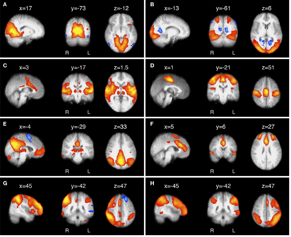
An example of resting-state networks. Each panel shows a distributed system whose time series tend to intercorrelate at rest, identified using independent components analysis. (Figure 28.1 from the book. © the authors and MIT Press; reproduced with permission — not covered by this site’s CC-BY license.)
A note of caution about naming: networks are often given psychological labels — the “salience network,” the “dorsal attention network” — but these labels invite problematic reverse inference (Chapter 7). A network contains billions of neurons with diverse functional properties and participates in many processes incompatible with any one-word label. Observing that a “salience” network is active does not license the conclusion that a participant is processing salience. For this reason, neuroanatomical labels (e.g., “cingulo-opercular network”) are increasingly preferred.
Rest has enormous practical appeal. Scans of 6–12 minutes suffice to identify group-level networks (reliability improves up to ~9–13 minutes of data), require no stimulus-delivery or response equipment, and can be run in clinical settings — which is why open repositories now contain resting-state data from tens of thousands of participants (HCP, ABCD, UK Biobank, ENIGMA, ABIDE, and others). The hopes are that resting connectivity will yield markers of aging, psychopathology, and clinical symptoms; guide brain stimulation targets; and support precision functional mapping — identifying functional areas within individuals, which requires much more data per person (40–90+ minutes). But rest has real pitfalls. Cognition is completely unconstrained: different people (and the same person at different moments) engage in different thoughts, and different connectivity patterns track different types of spontaneous thought. Wakefulness drifts — one study found that about half of resting participants are asleep after 10 minutes, and the transition to sleep changes activity patterns drastically. And some coherent “connectivity” reflects head motion, respiration, and cardiac pulsation rather than neural activity. Whether a given resting-state finding reflects intrinsic architecture, mental state, or physiological artifact is often genuinely hard to determine.
Table 1:A sample of large open resting-state datasets and how much resting data each acquires per person. Sample sizes are approximate. (Adapted from Table 28.1 in the book.)
| Study | Resting time per person | Sample |
|---|---|---|
| HCP | 60 min | ~1,200 healthy US adults |
| dHCP | 26 min | ~1,300 US participants, ages 5–21 |
| ABCD | 20 min | ~10,000 US adolescents |
| UK Biobank | 6 min | ~100,000 UK adults |
| ENIGMA | 4–15 min | ~60,000 across contributing studies |
| ABIDE / ABIDE II | 5–8 min | ~2,150 autistic individuals |
Naturalistic designs occupy a middle ground. A movie or story is not experimentally manipulated — these are observational designs — but it exposes everyone to the same rich sequence of visual, auditory, linguistic, social, and emotional events, engaging beliefs and expectations across multiple time scales. This shared time-locking enables analyses that rest cannot support. The most fundamental is inter-subject correlation (ISC): directly correlating time series across individuals, region by region. Where activity is driven by the shared stimulus, time courses align across people and ISC is high; where activity reflects idiosyncratic thought or noise, ISC is near zero. ISC requires no model of individual events or HRFs — the other subjects’ brains serve as the “model.” During rest there is no shared stimulus, so ISC provides a natural null benchmark. Beyond ISC, naturalistic data support encoding and decoding models that predict brain responses from stimulus features (and can partially reconstruct what a person is seeing), comparisons between brain representations and artificial neural network layers, and functional alignment methods such as hyperalignment (Chapters 30 and 38 develop these tools). Notably, connectivity measured during movie watching tends to be more reliable, and more predictive of behavior and cognitive performance, than connectivity measured at rest.
Hands-on tutorial
In this tutorial you will simulate the two paradigms and analyze them the way the field does: compute a functional connectivity matrix from resting multi-ROI time series, then use a shared “movie” stimulus to compute inter-subject correlation. The full labs add the cautionary tale: how motion spikes and vigilance drift inflate connectivity.
Step 1 — Simulate resting ROI time series and compute functional connectivity. We build eight ROIs organized into two networks: each ROI’s signal mixes a slow network-level fluctuation with ROI-specific noise. The correlation matrix recovers the block structure — the essence of every resting-state connectivity analysis.
% Simulate 2 networks x 4 ROIs at rest (10 min, TR = 2)
% Adapted from CANlab tutorials (github.com/canlab)
rng(28);                                % seed for reproducibility
TR = 2; n_t = 300; n_roi = 8;           % TR (s), volumes (10 min), regions (4 per network)
network = [1 1 1 1 2 2 2 2];            % network membership

kern    = exp(-0.5 * ((-4:4)' ./ 2) .^ 2); kern = kern ./ sum(kern);
smoothz = @(z) zscore(conv(z, kern, 'same'));   % slow (low-frequency) noise
net_sig = [smoothz(randn(n_t, 1)) smoothz(randn(n_t, 1))];

Y = zeros(n_t, n_roi);
w = 0.7;                                 % network signal weight
for i = 1:n_roi
    Y(:, i) = w * net_sig(:, network(i)) + ...
              (1 - w) * smoothz(randn(n_t, 1));
end
Y = zscore(Y);

FC = corr(Y);                            % functional connectivity matrix
figure; imagesc(FC, [-1 1]); axis square; colorbar
title('Resting-state functional connectivity');
% With real data: obj = fmri_data(fname); r = extract_roi_averages(obj, atlas_obj);
import numpy as np, matplotlib.pyplot as plt
# Simulate 2 networks x 4 ROIs at rest (10 min, TR = 2)
rng = np.random.default_rng(28) # seed for reproducibility
n_t, n_roi = 300, 8 # n_t = volumes (10 min at TR = 2 s), n_roi = regions (4 per network)
network = np.array([0, 0, 0, 0, 1, 1, 1, 1]) # network membership
kern = np.hanning(9); kern /= kern.sum() # slow fluctuations
smooth = lambda z: np.convolve(z, kern, mode="same")
net_sig = np.column_stack([smooth(rng.standard_normal(n_t))
for _ in range(2)])
w = 0.7 # network signal weight
Y = np.column_stack([w * net_sig[:, network[i]]
+ (1 - w) * smooth(rng.standard_normal(n_t))
for i in range(n_roi)])
Y = (Y - Y.mean(0)) / Y.std(0)
FC = np.corrcoef(Y.T) # functional connectivity
plt.imshow(FC, vmin=-1, vmax=1, cmap="RdBu_r"); plt.colorbar()
plt.title("Resting-state functional connectivity")Example output:
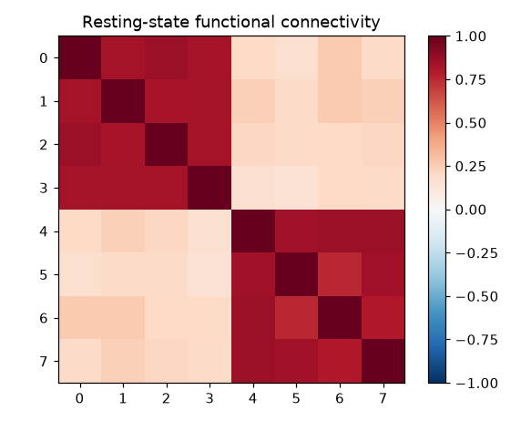
The correlation matrix recovers the built-in two-network block structure: strong within-network correlations (ROIs 1–4 and 5–8) and weak between-network ones.
Step 2 — Inter-subject correlation: movie vs. rest. Now we simulate ten “subjects” viewing the same movie: everyone’s ROI receives the same slow stimulus-driven time course plus idiosyncratic noise. For each subject , leave-one-out ISC correlates that subject’s regional time series with the average of the other subjects’ time series, where is the number of subjects:
ISCₛ — leave-one-out inter-subject correlation for subject s · yₛ — subject s’s time series in a given region · N — number of subjects
where is the leave-one-out inter-subject correlation for subject , the time series of a given region in subject , and the number of subjects; the average omits subject .
ISC is high during the movie — the shared stimulus aligns everyone’s time series — and near zero at rest, where there is nothing shared to align to.
% Shared "movie" drive + idiosyncratic noise, 10 subjects
n_sub = 10;                              % number of subjects
movie_sig = smoothz(randn(n_t, 1));      % shared stimulus time course

Y_movie = 0.6 * repmat(movie_sig, 1, n_sub) + ...   % 60% shared, 40% idiosyncratic
          0.4 * cell2mat(arrayfun(@(s) smoothz(randn(n_t, 1)), ...
                1:n_sub, 'UniformOutput', false));
Y_rest  = cell2mat(arrayfun(@(s) smoothz(randn(n_t, 1)), ...
                1:n_sub, 'UniformOutput', false));  % nothing shared

isc = @(Y) arrayfun(@(s) corr(Y(:, s), ...
      mean(Y(:, setdiff(1:n_sub, s)), 2)), 1:n_sub);  % leave-one-out ISC

fprintf('Mean ISC: movie = %3.2f, rest = %3.2f\n', ...
    mean(isc(Y_movie)), mean(isc(Y_rest)));
# Shared "movie" drive + idiosyncratic noise, 10 subjects
n_sub = 10 # number of subjects
movie_sig = smooth(rng.standard_normal(n_t)) # shared stimulus drive
noise = lambda: np.column_stack([smooth(rng.standard_normal(n_t))
for _ in range(n_sub)])
Y_movie = 0.6 * movie_sig[:, None] + 0.4 * noise() # 60% shared, 40% idiosyncratic
Y_rest = noise() # nothing shared
def isc(Y): # leave-one-out ISC
return np.array([np.corrcoef(Y[:, s],
np.delete(Y, s, axis=1).mean(1))[0, 1]
for s in range(Y.shape[1])])
print(f"Mean ISC: movie = {isc(Y_movie).mean():.2f}, "
f"rest = {isc(Y_rest).mean():.2f}")Example output:
Mean ISC: movie = 0.81, rest = -0.03The movie condition should show a mean ISC near 0.8, and rest near zero — the shared stimulus is what synchronizes brains. The full labs go further: they add motion spikes and a vigilance/arousal drift to the simulations and show how both inflate functional connectivity — including a spurious “group difference” between drowsy and alert subjects — and how scrubbing and nuisance regression help.
Open the full Python lab notebook → or download the MATLAB live script, which mirrors it using CANlab-style idioms.


Thought questions
Resting-state connectivity differences between a patient group and controls could reflect intrinsic network architecture, differences in what participants think about during the scan, differences in wakefulness, or differences in head motion and physiology. Design a study protocol — acquisition choices, monitoring, and analyses — that would help you distinguish among these interpretations.
The chapter cautions against psychological network labels like “salience network.” Connect this to reverse inference: what exactly is the fallacy when a clinical paper concludes that patients “process threat as more salient” because a network labeled salience shows altered connectivity? What kind of evidence would strengthen such a claim?
Naturalistic viewing is described as a middle ground between task and rest: more constrained than rest, more ecologically valid than isolated trials, but observational rather than experimental. For a research question of your choosing, argue which of the three paradigms you would use and what inferential price you pay for that choice.
ISC treats other participants’ brains as the model, requiring no event timing or HRF assumptions. What kinds of brain responses will ISC systematically miss, even when they are strongly stimulus-driven? (Consider idiosyncratic interpretations, individual timing differences, and responses that differ in sign across people.)
Scan length recommendations differ sharply: ~6–12 minutes suffices for group-level network identification, but 40–90+ minutes per person is desirable for precision functional mapping. Why should the amount of data needed depend so strongly on whether the target of inference is a group average or an individual brain?
Quiz yourself
Q1. What do participants do during a typical resting-state fMRI scan, and how long is a typical scan?
Answer: They lie in the scanner performing no overt task — usually keeping their eyes open and fixating a cross (sometimes eyes closed). Typical resting-state runs last about 6–12 minutes per subject.
Q2. What did Biswal et al. (1995) observe, and why was it important?
Answer: They found that BOLD time courses in left and right sensorimotor cortex were highly correlated at rest, suggesting that much of the apparent “noise” was coherent spontaneous activity. This discovery launched the field of resting-state functional connectivity.
Q3. What is the default mode network, and what kinds of tasks activate it above resting levels?
Answer: The DMN is a set of functionally connected regions — including ventromedial/dorsomedial prefrontal cortex, posterior cingulate, medial temporal lobe, and superior temporal cortex — that show high activity at rest and deactivate during many external tasks. It activates above resting levels during internally focused tasks: semantic memory retrieval, imagining the future, self-reflection, thinking about others’ minds, emotional experience, and mind-wandering.
Q4. How are resting-state networks typically identified from the data?
Answer: Either by clustering approaches based on pairwise correlations between voxel or region time series, or by data-decomposition algorithms such as independent components analysis (ICA) or PCA, in which voxels loading highly on the same component are taken to form a network. Typical solutions identify roughly 7–100 networks.
Q5. Give two reasons the book recommends against psychological labels like “salience network.”
Answer: (1) Such labels invite reverse inference — assuming that network activation implies engagement of that psychological process. (2) These networks contain billions of neurons with diverse functional properties and participate in many processes incompatible with a single psychological label, so neuroanatomical names are preferred.
Q6. Name three factors that can produce coherent resting-state “connectivity” that does not reflect ongoing neural interactions of interest.
Answer: Head motion artifacts, physiological noise (respiration and cardiac pulsation), and changes in wakefulness/arousal — notably, roughly half of resting participants are asleep after 10 minutes, and sleep drastically changes activity patterns. Unconstrained variation in spontaneous thought adds a further interpretive ambiguity.
Q7. What is inter-subject correlation (ISC), and what assumption does it avoid that standard GLM analysis requires?
Answer: ISC is the direct correlation of time series across individuals experiencing the same naturalistic stimulus; regions driven by the shared stimulus show synchronized time courses across people. It requires no model of individual stimulus events or an assumed HRF — the other subjects’ responses serve as the reference — so it maps shared, stimulus-locked activity without specifying what in the stimulus drives it.
Q8. Compared with resting-state connectivity, what advantages have been reported for connectivity measured during naturalistic viewing?
Answer: Connectivity during naturalistic fMRI has been found to be more reliable and more predictive of external behaviors and cognitive performance than resting-state connectivity, while also constraining participants’ mental states more than rest does.
 The book: Elements of Functional Magnetic Resonance Imaging — Wager & Lindquist, MIT Press