Statistical Power and Sample Size
Run this code: ⚡ In-browser lab · Colab · MATLAB Online
Overview
Power analysis is a study planning tool: it is performed before data collection, to choose a sample size and design that give a good chance of detecting the effects you care about. In fMRI this is complicated because power depends on many factors — the psychological manipulation, task design, acquisition hardware, preprocessing, and analysis choices — and it differs across brain regions. Fortunately, all of these influences converge on a “final common pathway”: the effect size in the group analysis. If you can specify the effect size you expect, or the minimum effect you would like to be able to detect, then power and sample size calculations become straightforward and can be done with standard tools (or a few lines of code, as in the labs below).
Effect sizes are unit-free descriptions of how large an effect is, independent of sample size. Cohen’s divides a mean effect by its standard deviation — for a one-sample test, , where is the mean effect and its standard deviation across participants — and benchmark values of = 0.2, 0.5, and 0.8 are conventionally called small, medium, and large. Pearson’s plays the same role for brain–behavior correlations, and the two are interconvertible:
r — effect size expressed as a Pearson correlation · d — Cohen’s standardized mean difference
where is the effect size expressed as a Pearson correlation and is Cohen’s standardized mean difference; both are unit-free.
Crucially, effect size is distinct from statistical significance. Test statistics and P values depend on sample size: with a large enough sample size , arbitrarily small — and practically meaningless — effects become “significant.” Effect sizes, by contrast, speak to practical importance, replicability, and the sample sizes future studies will need. For a one-sample t-test the two are linked by , so an observed t-statistic can be converted back into an effect size estimate () — a trick used throughout the labs.
There is a catch, however: typical neuroimaging studies are poorly suited to estimating effect sizes. A mass-univariate analysis tests 50,000–350,000 voxels and then reports effect sizes only for the small subset that survived thresholding. Voxels reach significance when they have true signal and noise that happens to favor the hypothesis, so the selected voxels’ estimated effects are biased upward — like a mediocre golfer reporting only his 10 best holes. This selection bias, or “winner’s curse,” grows worse with more tests, smaller samples, and smaller true effects — and, counterintuitively, more stringent correction for multiple comparisons increases the inflation, because only the luckiest noise survives. The same logic underlies P-hacking, HARKing, and circular (“double-dipping”) analyses: selecting, weighting, or sorting results in a way that depends on the test outcome short-circuits inference. Remedies include pre-registration and Registered Reports, and — increasingly practical in neuroimaging — discovery–validation designs that lock in a region, network, or multivariate pattern in one sample and test that single effect in an independent sample, yielding unbiased effect size estimates.
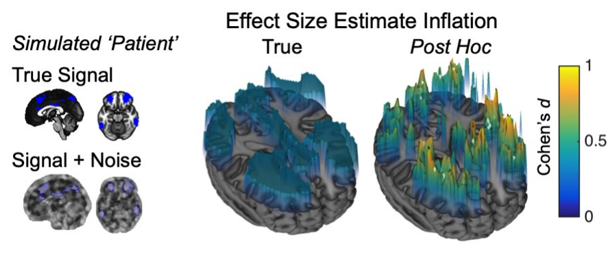
Selection bias in action. Voxels in blue were assigned a true effect of Cohen’s , and spatially correlated noise was added for each of 30 simulated participants. After a group t-test thresholded at P < 0.001, every significant voxel’s estimated effect size (right, “Post Hoc”) exceeds the true value (center, “True”) — because voxels whose noise favors the hypothesis are selected, and the rest are discarded. (Figure 29.1 from the book. © the authors and MIT Press; reproduced with permission — not covered by this site’s CC-BY license.)
Statistical power is the probability of rejecting the null hypothesis when it is false — of detecting a true effect if it exists. Power increases with the true effect size and with sample size, and decreases as the significance threshold becomes more stringent. This last point is where multiplicity exacts its price: correcting for multiple comparisons across the brain pushes the effective per-test alpha from 0.05 down to roughly 0.001 (a level that often approximates FDR q < 0.05) or to ~4 × 10⁻⁶ (typical familywise error control with permutation tests). The power curves below quantify the cost. Detecting a brain–behavior correlation of with 80% power requires about N = 28 in a single a priori ROI, N = 53 at P < 0.001, and N = 100 or more with FWER correction. For a small effect of , the corresponding numbers are N = 781, N = 1,537, and nearly N = 3,000. Comparing two groups roughly quadruples the total sample needed relative to a one-sample test. As a planning anchor, a reasonable expectation for task effects in individual voxels is (based on a reference set of Human Connectome Project task activations): detecting it in a single ROI requires N = 34, and with FWER control approximately N = 121 — while a two-group comparison with FWER control requires roughly N = 466.
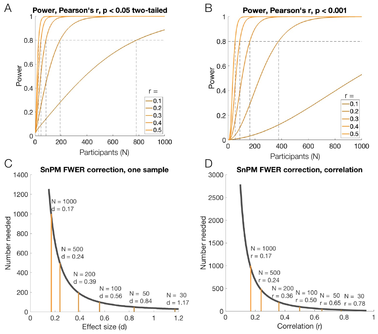
Power curves as a function of effect size and sample size. (A) Power for a single test at P < 0.05 two-tailed: detecting = 0.1–0.5 with 80% power requires N = 781, 193, 84, 46, and 28. (B) At P < 0.001 (often approximating FDR correction), the required samples roughly double: N = 1,537, 378, 163, 88, and 53. (C, D) Sample size needed for 80% power with permutation-based FWER correction, for one-sample tests (d) and correlations (r). (Figure 29.2 from the book. © the authors and MIT Press; reproduced with permission — not covered by this site’s CC-BY license.)
These sobering numbers frame the modern power failure debate. Underpowered studies not only miss true effects; their “significant” findings are more likely to be false positives, and the effects that do survive are inflated by the winner’s curse — a recipe for irreplicable findings. The problem is most acute for Brain-Wide Association Studies (BWAS) linking individual differences in brain measures to behavior. Marek, Tervo-Clemmens and colleagues (2022) analyzed tens of thousands of participants and found that the largest brain–behavior correlations in single voxels or edges were around — requiring hundreds to thousands of participants for adequate power. But the story has a constructive coda: with appropriate multivariate models that aggregate signal across the brain, effects up to about are attainable in the same data, cutting required samples roughly 16-fold and bringing individual-differences prediction within reach of samples in the hundreds. Task-based states and decoding analyses can yield much larger effects still (multivariate patterns can exceed ), permitting detection in small samples.
Finally, power is not just about the number of participants: the amount and quality of data per participant matter too. With a fixed scanning budget, the optimal allocation depends on the ratio of between-subject variance () to within-subject variance (). Large — true individual differences — favors more participants; large — noisy within-person measurements — favors longer scans. For typical group analyses, between-subject variance is rate-limiting, so the rule of thumb is: scan as many participants as possible, with at least ~30 minutes of functional time each. An empirical analysis of a working memory study (below) found that 40 total scan hours were best spent on ~38–40 participants scanned for about an hour each. For studies predicting individual-level outcomes, or in homogeneous-population designs like visual psychophysics, deeper scanning of fewer participants can be preferable. When in doubt, larger samples are better — with only 40 subjects and FWER correction, power was around 10% even for a robust working memory contrast.
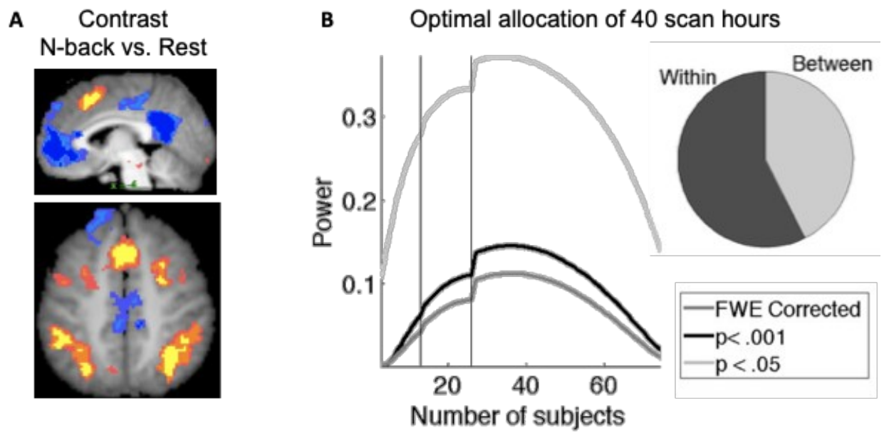
Balancing scan time and number of subjects. (A) Contrast map for an N-back working memory task. (B) Power as a function of sample size given a fixed budget of 40 total scan hours, for three thresholds. Within- and between-subject variance were roughly balanced (pie chart); the maximum-power solution is ~38 subjects scanned for about one hour each. (Figure 29.3 from the book. © the authors and MIT Press; reproduced with permission — not covered by this site’s CC-BY license.)
Hands-on tutorial
In this tutorial you will build a power calculator from scratch and use it to answer the planning questions above: How many participants do I need? What is the smallest effect I can detect? And how badly will the winner’s curse inflate my post hoc effect sizes? The calculations mirror the simulation code behind the book’s power figures (github.com/canlab).
Step 1 — Analytic power curves. Power for a one-sample t-test comes from the noncentral t distribution: with true effect and sample size , the t-statistic is distributed with noncentrality , and power is the probability that it exceeds the critical value . One convention to fix up front: a planned test is two-tailed, while thresholds applied to statistic maps (“”) are conventionally directional, so we carry a tails argument.
% Power for a one-sample t-test (requires Statistics Toolbox)
% Adapted from power_calc.m in the CANlab tools (github.com/canlab)
d     = 0.5;    % true effect size (Cohen's d; 0.5 = "medium")
alpha = .05;    % significance level for the planned test
tails = 2;      % 2 = two-tailed planned test; 1 = directional map threshold
N     = 2:200;  % range of sample sizes to evaluate

tcrit = tinv(1 - alpha/tails, N - 1);    % critical t (tails = 1 for maps)
delta = d .* sqrt(N);                    % noncentrality parameter
pow   = 1 - nctcdf(tcrit, N - 1, delta); % power at each N

ncrit = N(find(pow >= .80, 1));          % N needed for 80% power
fprintf('d = %.1f: N = %d for 80%% power at p < %.2f\n', d, ncrit, alpha)

figure; plot(N, pow, 'LineWidth', 2); hold on
plot([2 200], [.8 .8], 'k--')
xlabel('Sample size (N)'); ylabel('Power')
import numpy as np
import matplotlib.pyplot as plt
from scipy import stats
def power_one_sample(d, n, alpha=0.05, tails=2):
"""Power of a one-sample t-test with true effect size d.
tails=2 for a planned test; tails=1 for directional map thresholds."""
df = n - 1
t_crit = stats.t.ppf(1 - alpha / tails, df)
return 1 - stats.nct.cdf(t_crit, df, d * np.sqrt(n))
d, alpha = 0.5, 0.05 # d = true effect size ("medium"); alpha = significance level
N = np.arange(2, 201) # range of sample sizes to evaluate
pow_curve = power_one_sample(d, N, alpha)
n_crit = N[np.argmax(pow_curve >= 0.80)] # N needed for 80% power
print(f"d = {d}: N = {n_crit} for 80% power at p < {alpha}")
plt.plot(N, pow_curve); plt.axhline(0.8, ls="--", c="k")
plt.xlabel("Sample size (N)"); plt.ylabel("Power")Example output:
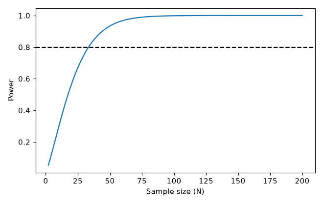
Power rises steeply with sample size and crosses the 80% criterion (dashed line) at N = 34 for a medium effect of .
d = 0.5: N = 34 for 80% power at p < 0.05Repeating this across effect sizes and alpha levels reproduces the book’s power curves — and shows the multiplicity tax directly: the same effect that needs N = 34 at P < 0.05 needs roughly N = 122 under whole-brain FWER correction, and about 460 participants if the question is a patient–control difference. Inverted, the same code reconstructs Figure 29.2C/D from scratch: with FWER correction, N = 30 buys 80% power only for , and N = 100 only for .
Step 2 — The winner’s curse. Simulate many “voxels” that all share the same true effect (), threshold the map, and compare post hoc effect sizes in significant voxels with the truth.
% Simulate 20,000 voxels, all with true d = 0.5, N = 30 subjects
% Concept from effect_size_inflation_example_sim.m (github.com/canlab)
rng(29);          % fix the random seed for reproducibility
n      = 30;      % n = participants per simulated study
nvox   = 20000;   % nvox = number of simulated voxels (tests)
d_true = 0.5;     % true effect size in EVERY voxel

dat  = d_true + randn(n, nvox);          % subjects x voxels
[~, ~, ~, st] = ttest(dat);              % group t-test at each voxel
p_dir = 1 - tcdf(st.tstat, n - 1);       % directional p, as in mapping
d_hat = st.tstat ./ sqrt(n);             % observed effect sizes

sig = p_dir < .001;                      % mapping threshold (uncorrected)
fprintf('True d = %.2f | mean d-hat: all voxels %.2f, significant only %.2f\n', ...
    d_true, mean(d_hat), mean(d_hat(sig)))
# Simulate 20,000 voxels, all with true d = 0.5, N = 30 subjects
rng = np.random.default_rng(29) # fixed seed for reproducibility
n, nvox, d_true = 30, 20000, 0.5 # n = participants; nvox = voxels (tests); d_true = true effect everywhere
dat = d_true + rng.standard_normal((n, nvox)) # subjects x voxels
t, _ = stats.ttest_1samp(dat, 0.0)
p_dir = stats.t.sf(t, n - 1) # directional p, as in mapping
d_hat = t / np.sqrt(n) # observed effect sizes
sig = p_dir < 0.001 # mapping threshold (uncorrected)
print(f"True d = {d_true} | mean d-hat: all voxels {d_hat.mean():.2f}, "
f"significant only {d_hat[sig].mean():.2f}")Example output:
True d = 0.5 | mean d-hat: all voxels 0.51, significant only 0.76Every voxel has the same true effect, yet the significant subset averages — about 50% inflation, and the bias worsens at stricter thresholds or smaller N (at with N = 15, the surviving voxels average , four times the truth). The full labs go further: power for correlations via the Fisher z transform, one- and two-group sample sizes under Bonferroni/FDR/FWER-level alphas, minimum detectable effect sizes for a planned N, and a reanalysis of the univariate-vs-multivariate power gap highlighted by the BWAS debate.
Open the full Python lab notebook → or download the MATLAB live script, which mirrors it using CANlab-style power utilities.


Thought questions
Stricter multiple comparisons correction reduces false positives but increases the inflation of post hoc effect sizes among surviving voxels. Explain why both statements are true simultaneously, and what this implies for using published whole-brain results to plan a new study’s sample size.
A colleague argues that small-sample studies are self-correcting: “If we found it with N = 15, the effect must be huge, so it’s the effects worth caring about.” Using the concepts of power, confidence interval width, and the winner’s curse, construct the counterargument — and identify any circumstances in which your colleague might have a point (e.g., multivariate task decoding with ).
The Marek et al. (2022) BWAS findings ( for univariate brain–behavior correlations) triggered calls for consortium-scale samples, yet multivariate models achieve in the same data. How should these two facts jointly shape the design of an individual-differences study with a budget for 300 participants? Consider what is gained and lost by moving from voxel-level maps to predictive patterns.
You have 60 hours of scanner time for a group study of a cognitive task. Using the concepts of within-subject variance () and between-subject variance (), describe how you would decide between 60 participants × 1 hour and 20 participants × 3 hours — and how your answer would change if the goal were instead to build a within-person predictive model, or to study a rare patient population.
Pre-registration and discovery–validation designs both aim to eliminate selection bias, but they make different tradeoffs between analytic flexibility and inferential rigor. For a new fMRI study of emotion regulation in adolescents, sketch a workflow that preserves the ability to make data-driven methodological choices while still delivering an unbiased effect size estimate for the primary hypothesis.
Quiz yourself
Q1. What is statistical power?
Answer: Power is the probability of rejecting the null hypothesis when it is false — that is, the probability of detecting a true effect if it exists. It increases with larger true effect sizes and larger samples, and decreases with more stringent significance thresholds.
Q2. How does an effect size like Cohen’s differ from a t-statistic or P value?
Answer: Cohen’s is a unit-free, sample-size-independent description of an effect’s magnitude (mean effect divided by standard deviation). Test statistics and P values depend on sample size and reflect statistical significance, not magnitude — with a large enough N, even tiny, practically unimportant effects become significant. The two are related by for a one-sample test.
Q3. What is the “winner’s curse” in neuroimaging, and what three factors make it worse?
Answer: When effect sizes are reported only for voxels that survived thresholding, the estimates are biased upward, because voxels are selected partly for having favorable noise. The bias grows with (1) more tests (voxels) conducted, (2) smaller samples, and (3) smaller true effects. Stricter statistical thresholds also increase the inflation among surviving voxels.
Q4. Roughly how many participants are needed to detect a brain–behavior correlation of r = 0.5 with 80% power in (a) one a priori ROI at P < 0.05, (b) at P < 0.001, and (c) with whole-brain FWER correction?
Answer: Approximately (a) N = 28 for a single ROI, (b) N = 53 at P < 0.001 (a level that often approximates FDR correction), and (c) N = 100 or more for FWER control. Requirements grow dramatically for smaller effects — r = 0.1 needs N = 781 for even a single test.
Q5. What is the rule of thumb for sample sizes when comparing two groups (e.g., patients vs. controls) rather than testing one group?
Answer: You need approximately 4 times the total sample size for a between-group comparison. For example, an effect of d = 0.4 detectable with N = 50 in a one-sample test requires about N = 101 per group (~200 total) for 80% power in a two-group comparison.
Q6. Why are pre-registration and discovery–validation approaches effective against selection bias?
Answer: Both lock down which effect is tested and how, before the confirmatory test is run. Testing a single pre-specified effect (a region, network, or multivariate pattern) in an independent sample eliminates the dependence between selection criteria and test outcome (circularity), so the false positive rate is controlled and the replication-sample effect size is an unbiased estimate of the true effect.
Q7. What did the Marek et al. (2022) BWAS analyses find, and what is the multivariate counterpoint?
Answer: Across large-scale datasets, the largest univariate brain–behavior correlations were only about r = 0.1, implying that hundreds to thousands of participants are needed for reliable voxel- or edge-level individual-differences findings. However, multivariate models aggregating signal across the brain can reach about r = 0.4 in the same data — reducing required sample sizes roughly 16-fold and making prediction feasible with samples in the hundreds.
Q8. With a fixed total scanning budget, when should you favor more participants versus more scan time per participant?
Answer: The balance depends on the ratio of between-subject to within-subject variance. When between-subject variance dominates (typical for group analyses of cognitive and affective tasks), add participants — with at least ~30 minutes of functional time each. When within-subject variance dominates, or for predicting individual-level outcomes, longer or repeated scans per person become more valuable. Empirically, one working memory study found ~40 hours best allocated as ~1 hour each for ~38–40 participants.
 The book: Elements of Functional Magnetic Resonance Imaging — Wager & Lindquist, MIT Press