Chapter 29 Lab — Statistical Power and Sample Size (Python) - Elements of fMRI Analysis

In this lab you will build an fMRI power calculator from first principles and use it to answer the questions every study proposal must face: How many participants do I need? What is the smallest effect I can detect? And how much will the “winner’s curse” inflate my post hoc effect sizes? We compute power analytically from the noncentral t distribution, verify it by simulation, quantify the cost of multiple comparisons correction, and reproduce the core of the univariate-vs-multivariate power argument from the BWAS debate (Marek et al., 2022).

How to run this: This notebook runs in the browser (Pyodide), on Colab, or locally — it uses only numpy, scipy, and matplotlib on simulated data, and every cell runs in seconds. It accompanies the Chapter 29 tutorial page.

Calculations mirror the CANlab power utilities and simulation scripts behind the book’s figures (github.com/canlab).

▶ This notebook is interactive. Click the ⏻ power icon at the top right of this page to run it in your browser — no installation needed (the kernel takes ~30–60 s to start the first time). Then run cells top to bottom, starting with the first code cell below: later cells depend on the imports and variables defined earlier, and will error if you skip ahead.

import numpy as np
import matplotlib.pyplot as plt
from scipy import stats

rng = np.random.default_rng(29)      # fixed random seed for reproducibility
plt.rcParams["figure.dpi"] = 90      # modest figure resolution for in-browser rendering

Step 1 — Power for a one-sample t-test, analytically¶

For a one-sample t-test with true effect size $d = \mu/\sigma$ and sample size $N$ , the test statistic follows a noncentral t distribution with $N-1$ degrees of freedom and noncentrality parameter $\delta = d\sqrt{N}$ . Power is the probability that this statistic exceeds the critical value:

\text{power} = 1 - F_{nct}\!\left(t_{crit};\; N-1,\; d\sqrt{N}\right)

(1)

F_nct — noncentral t cumulative distribution function · t_crit — critical t value at level α · N − 1 — degrees of freedom · d√N — noncentrality parameter δ

where $F_{nct}$ is the cumulative distribution function of the noncentral t distribution, $t_{crit}$ the critical value at significance level $\alpha$ , $N-1$ the degrees of freedom, $d$ the true effect size, and $d\sqrt{N}$ the noncentrality parameter $\delta$ .

For a two-sample (balanced) comparison, $\delta = d\sqrt{n/2}$ with $n$ per group and $df = 2n - 2$ — which is why group comparisons need roughly 4× the total sample. For correlations we use the Fisher z approximation: $\text{atanh}(r)$ is approximately normal with standard error $1/\sqrt{N-3}$ .

One convention to fix up front: a planned test is usually two-tailed ( $\alpha$ split between tails), whereas thresholds applied to fMRI statistic maps (“ $p < .001$ ”) are conventionally directional — one tail, because we threshold positive activations. Our functions take a tails argument so we can follow that convention and reproduce the book’s reference numbers.

def power_one_sample(d, n, alpha=0.05, tails=2):
    """Power of a one-sample t-test with true effect size d.

    tails=2 for a two-sided planned test; tails=1 for the directional
    thresholds conventionally applied to fMRI statistic maps.
    """
    n = np.asarray(n, dtype=float)
    df = n - 1
    t_crit = stats.t.ppf(1 - alpha / tails, df)
    return 1 - stats.nct.cdf(t_crit, df, d * np.sqrt(n))

def power_two_sample(d, n_per_group, alpha=0.05, tails=2):
    """Power of a two-sample t-test, balanced groups of size n_per_group."""
    n = np.asarray(n_per_group, dtype=float)
    df = 2 * n - 2
    t_crit = stats.t.ppf(1 - alpha / tails, df)
    return 1 - stats.nct.cdf(t_crit, df, d * np.sqrt(n / 2))

def power_correlation(r, n, alpha=0.05, tails=2):
    """Power to detect a correlation r, Fisher z approximation."""
    n = np.asarray(n, dtype=float)
    z_crit = stats.norm.ppf(1 - alpha / tails)
    return stats.norm.cdf(np.sqrt(n - 3) * np.arctanh(r) - z_crit)

def n_for_power(power_fn, effect, alpha=0.05, tails=2, target=0.80, n_max=6000):
    """Smallest N (or n per group) achieving the target power."""
    n = np.arange(3, n_max)
    pow_curve = power_fn(effect, n, alpha, tails)
    idx = np.argmax(pow_curve >= target)
    return int(n[idx]) if pow_curve[idx] >= target else None

# Quick check against benchmark values
for d in [0.2, 0.5, 0.8]:
    print(f"d = {d}: N = {n_for_power(power_one_sample, d):>4d} "
          f"for 80% power (one-sample, p < .05 two-tailed)")

d = 0.2: N =  199 for 80% power (one-sample, p < .05 two-tailed)
d = 0.5: N =   34 for 80% power (one-sample, p < .05 two-tailed)
d = 0.8: N =   15 for 80% power (one-sample, p < .05 two-tailed)

A “medium” effect of $d = 0.5$ needs about N = 34 — matching standard power software (e.g., G*Power). Now draw the classic power curves: power as a function of $N$ for several effect sizes.

d_vals = [0.2, 0.3, 0.4, 0.5, 0.8]   # effect sizes (Cohen's d) to plot
N = np.arange(3, 251)                # range of sample sizes to evaluate

fig, ax = plt.subplots(figsize=(7, 4.5))
for d in d_vals:
    ax.plot(N, power_one_sample(d, N), label=f"d = {d}")
    n80 = n_for_power(power_one_sample, d)
    if n80 is not None and n80 <= N.max():
        ax.plot([n80, n80], [0, 0.8], ":", color="gray", lw=1)
ax.axhline(0.8, ls="--", color="k", lw=1)
ax.set(xlabel="Sample size (N)", ylabel="Power",
       title="One-sample t-test power, p < .05 two-tailed")
ax.legend(); ax.set_ylim(0, 1.02); plt.tight_layout()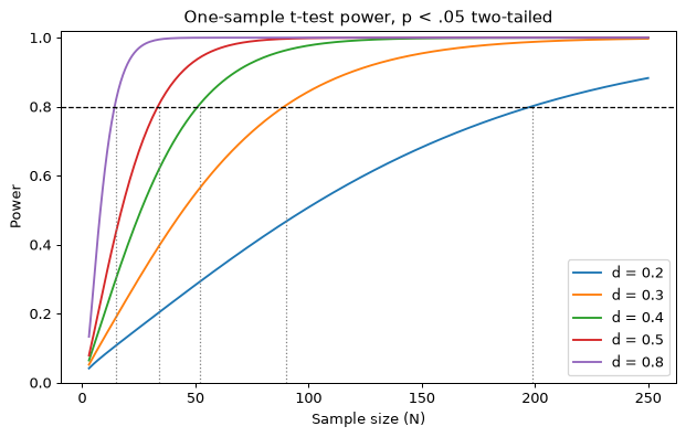

Each curve rises toward 1 as $N$ grows, but the sample size needed for 80% power (dotted drop lines) explodes as effects shrink: $d = 0.8$ needs ~15 participants, $d = 0.2$ needs ~199. Sanity check by simulation — power is just the long-run fraction of significant results, so we can verify the analytic curve with brute force.

def simulated_power(d, n, alpha=0.05, n_sims=2000):
    """Fraction of simulated one-sample experiments reaching p < alpha.

    n_sims = number of simulated experiments; more gives smoother estimates."""
    dat = d + rng.standard_normal((n_sims, n))      # n_sims experiments x n subjects
    t, p = stats.ttest_1samp(dat, 0.0, axis=1)
    return np.mean(p < alpha)

print(f"{'N':>4} {'analytic':>9} {'simulated':>10}")
for n in [10, 20, 34, 50, 80]:
    print(f"{n:>4} {power_one_sample(0.5, n):>9.3f} {simulated_power(0.5, n):>10.3f}")

   N  analytic  simulated
  10     0.293      0.300
  20     0.564      0.573
  34     0.808      0.806
  50     0.934      0.936
  80     0.993      0.994

Analytic and simulated power agree to within Monte Carlo error. From here on we trust the analytic formulas.

Step 2 — The cost of multiple comparisons¶

A mass-univariate analysis cannot use $\alpha = 0.05$ per voxel. Correction pushes the effective per-test threshold to roughly:

Threshold	Tails	Typical use
$p < 0.05$	2	one pre-registered ROI test
$p < 0.001$	1	uncorrected mapping; often approximates FDR $q < .05$
$p < 0.05/1000$	1	Bonferroni over ~1,000 parcels/tests
$p < 4.26\times 10^{-6}$	1	whole-brain FWER (permutation-based, empirical average)

How does the required sample size change across these thresholds — and how much worse is a two-group comparison?

# Each threshold: (label, per-test alpha, tails); tails=1 = directional map threshold
thresholds = [("p < .05, two-tailed (ROI)", 0.05, 2),
              ("p < .001 (~FDR q < .05)", 0.001, 1),
              ("Bonferroni, 1,000 tests", 0.05 / 1000, 1),
              ("FWER whole brain", 4.26e-6, 1)]

d_grid = [0.2, 0.3, 0.5, 0.8]   # effect sizes (Cohen's d) to tabulate
header = f"{'threshold':<26}" + "".join(f"  d={d:<5}" for d in d_grid)

print("N for 80% power, ONE-SAMPLE test (e.g., task activation vs. baseline)")
print(header)
for name, a, t in thresholds:
    row = [n_for_power(power_one_sample, d, alpha=a, tails=t) for d in d_grid]
    print(f"{name:<26}" + "".join(f"  {n:<6}" for n in row))

print("\nTOTAL N for 80% power, TWO-GROUP comparison (patients vs. controls)")
print(header)
for name, a, t in thresholds:
    row = [2 * n_for_power(power_two_sample, d, alpha=a, tails=t) for d in d_grid]
    print(f"{name:<26}" + "".join(f"  {n:<6}" for n in row))

N for 80% power, ONE-SAMPLE test (e.g., task activation vs. baseline)
threshold                   d=0.2    d=0.3    d=0.5    d=0.8

p < .05, two-tailed (ROI)   199     90      34      15    
p < .001 (~FDR q < .05)     392     177     67      29    
Bonferroni, 1,000 tests     568     257     98      43    
FWER whole brain            711     322     122     54    

TOTAL N for 80% power, TWO-GROUP comparison (patients vs. controls)
threshold                   d=0.2    d=0.3    d=0.5    d=0.8  
p < .05, two-tailed (ROI)   788     352     128     52

p < .001 (~FDR q < .05)     1552    692     254     102

Bonferroni, 1,000 tests     2248    1004    366     148

FWER whole brain            2812    1256    460     186

Reading down each column, correcting for multiplicity multiplies the required sample by ~3–4×: a medium effect ( $d = 0.5$ ) needs 34 participants for one ROI test but about 122 under whole-brain FWER correction. Reading across the two tables, the two-group comparison needs roughly 4× the total sample — 128 total for $d = 0.5$ at $p < .05$ , and about 460 with FWER correction. (These are the book’s planning numbers: N = 34, 121, 130, and 466.) The same logic applies to brain–behavior correlations:

r_grid = [0.1, 0.2, 0.3, 0.4, 0.5]   # correlation effect sizes, as in Figure 29.2

fig, axes = plt.subplots(1, 2, figsize=(11, 4.2), sharey=True)
N = np.arange(4, 2001)              # range of sample sizes to evaluate
panels = [("p < .05, two-tailed", 0.05, 2), ("p < .001, directional", 0.001, 1)]
for ax, (name, a, t) in zip(axes, panels):
    for r in r_grid:
        ax.plot(N, power_correlation(r, N, alpha=a, tails=t), label=f"r = {r}")
    ax.axhline(0.8, ls="--", color="k", lw=1)
    ax.set(xlabel="Participants (N)", title=f"Correlation power, {name}", xlim=(0, 1000))
axes[0].set_ylabel("Power"); axes[0].legend(loc="lower right")
plt.tight_layout()

print("N for 80% power to detect a correlation:")
print(f"{'r':>5} {'p<.05':>8} {'p<.001':>8} {'FWER':>8}")
for r in r_grid:
    ns = [n_for_power(power_correlation, r, alpha=a, tails=t)
          for a, t in [(0.05, 2), (0.001, 1), (4.26e-6, 1)]]
    print(f"{r:>5} " + " ".join(f"{n or '>6000':>8}" for n in ns))

N for 80% power to detect a correlation:
    r    p<.05   p<.001     FWER
  0.1      783     1539     2787
  0.2      194      380      685
  0.3       85      165      296
  0.4       47       90      160
  0.5       30       55       96

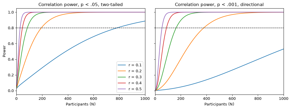
These reproduce the book’s Figure 29.2 reference values to within a participant or two: detecting $r = 0.5$ needs ~28 participants for a single ROI test, ~53 at $p < .001$ , and ~100 with FWER correction — while $r = 0.1$ needs roughly 780, 1,540, and 2,790. Small correlations and whole-brain search are a brutal combination.

Step 3 — Minimum detectable effect size¶

Power analysis can be inverted: given the sample size you can afford, what is the smallest effect you have an 80% chance of detecting? This minimum detectable effect size (MDES) is an honest summary of a study’s sensitivity — and a useful line for grant proposals.

def min_detectable_d(n, alpha, tails=2, target=0.80, d_grid=np.arange(0.05, 3.001, 0.005)):
    """Smallest one-sample d detectable with the target power at sample size n."""
    pow_curve = power_one_sample(d_grid, np.full_like(d_grid, n), alpha, tails)
    idx = np.argmax(pow_curve >= target)
    return d_grid[idx] if pow_curve[idx] >= target else np.nan

def min_detectable_r(n, alpha, tails=2, target=0.80, r_grid=np.arange(0.02, 0.9901, 0.002)):
    """Smallest correlation detectable with the target power at sample size n."""
    pow_curve = power_correlation(r_grid, np.full_like(r_grid, n), alpha, tails)
    idx = np.argmax(pow_curve >= target)
    return r_grid[idx] if pow_curve[idx] >= target else np.nan

n_grid = [30, 50, 100, 200, 500, 1000]   # affordable sample sizes to evaluate
print("Minimum detectable effect with 80% power (one-sample d | correlation r):")
print(f"{'N':>6} {'d, p<.05':>9} {'d, FWER':>9} {'r, p<.05':>10} {'r, FWER':>9}")
for n in n_grid:
    print(f"{n:>6} {min_detectable_d(n, .05):>9.2f}"
          f" {min_detectable_d(n, 4.26e-6, tails=1):>9.2f}"
          f" {min_detectable_r(n, .05):>10.2f}"
          f" {min_detectable_r(n, 4.26e-6, tails=1):>9.2f}")

Minimum detectable effect with 80% power (one-sample d | correlation r):
     N  d, p<.05   d, FWER   r, p<.05   r, FWER
    30      0.53      1.16       0.49      0.77
    50      0.40      0.83       0.39      0.65
   100      0.28      0.56       0.28      0.49

   200      0.20      0.38       0.20      0.36
   500      0.13      0.24       0.13      0.23
  1000      0.09      0.17       0.09      0.17

d_grid = np.arange(0.1, 1.21, 0.005)   # effect sizes to scan for the N-needed curve
n_needed = np.array([n_for_power(power_one_sample, d, alpha=4.26e-6, tails=1) or np.nan
                     for d in d_grid])

fig, ax = plt.subplots(figsize=(7, 4.5))
ax.plot(d_grid, n_needed, color="0.25", lw=3)
for n in [30, 50, 100, 200, 500, 1000]:
    mdes = min_detectable_d(n, 4.26e-6, tails=1)
    ax.plot([mdes, mdes], [0, n], color="orange", lw=2)
    ax.annotate(f"N = {n}\nd = {mdes:.2f}", (mdes, n), textcoords="offset points",
                xytext=(6, 8), fontsize=8)
ax.set(xlabel="Effect size (d)", ylabel="N needed for 80% power",
       title="Whole-brain FWER correction, one-sample test", ylim=(0, 1300))
plt.tight_layout()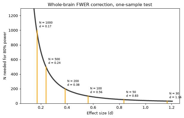

This panel is a from-scratch reconstruction of Figure 29.2C, and the drop-lines recover its annotations ( $N = 30 \rightarrow d \approx 1.17$ , $N = 100 \rightarrow d \approx 0.56$ , $N = 1000 \rightarrow d \approx 0.17$ ). The message: with whole-brain FWER correction, a typical N = 30 study is powered only for very large effects — far larger than the $d \approx 0.5$ typical of task effects in individual voxels. This is the quantitative heart of the “power failure” concern.

Step 4 — The winner’s curse: effect size inflation at a threshold¶

Now the other side of the coin. When we estimate effect sizes only in voxels that survived thresholding, the estimates are biased upward: voxels are selected partly because their noise favored the hypothesis. We simulate a brain-full of voxels all sharing the same true effect ( $d = 0.5$ , the true value in the book’s Figure 29.1 simulation) and compare post hoc estimates to the truth.

n_sub, n_vox, d_true = 30, 20000, 0.5   # n_sub = participants; n_vox = voxels (tests); d_true = true effect everywhere

dat = d_true + rng.standard_normal((n_sub, n_vox))     # subjects x voxels
t, _ = stats.ttest_1samp(dat, 0.0)
p_dir = stats.t.sf(t, n_sub - 1)                        # directional (one-tailed) p
d_hat = t / np.sqrt(n_sub)                              # observed effect size per voxel

sig = p_dir < 0.001                                     # mapping threshold (uncorrected)
print(f"True effect size:                 d = {d_true:.2f}")
print(f"Mean estimate, ALL voxels:        d = {d_hat.mean():.2f}   (unbiased)")
print(f"Mean estimate, significant only:  d = {d_hat[sig].mean():.2f}   "
      f"({100 * (d_hat[sig].mean() / d_true - 1):.0f}% inflated)")
print(f"Voxels significant at p < .001:   {sig.mean() * 100:.1f}%  "
      f"(analytic power: {100 * power_one_sample(d_true, n_sub, .001, tails=1):.1f}%)")

fig, ax = plt.subplots(figsize=(7, 4))
bins = np.linspace(-0.2, 1.4, 60)
ax.hist(d_hat, bins=bins, color="0.75", label="all voxels")
ax.hist(d_hat[sig], bins=bins, color="crimson", alpha=0.75,
        label="significant (p < .001)")
ax.axvline(d_true, color="k", ls=":", lw=2, label="true d = 0.5")
ax.set(xlabel=r"Estimated effect size ($\hat{d}$)", ylabel="Number of voxels",
       title="Winner's curse: selection inflates post hoc effect sizes")
ax.legend(); plt.tight_layout()

True effect size:                 d = 0.50
Mean estimate, ALL voxels:        d = 0.51   (unbiased)
Mean estimate, significant only:  d = 0.76   (52% inflated)
Voxels significant at p < .001:   28.5%  (analytic power: 28.3%)

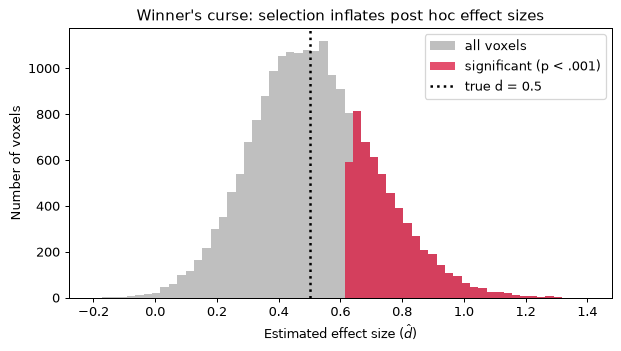
Every voxel has the same true effect, yet the significant subset (red) sits almost entirely to the right of the truth. Two factors govern the inflation — threshold stringency and sample size:

thresholds = [0.05, 0.005, 0.001, 4.26e-6]   # per-test alphas, lenient to FWER-level
sample_sizes = [15, 30, 60, 120]             # participants per simulated study

print(f"{'N':>5} " + "".join(f"  p<{a:<9.2g}" for a in thresholds))
for n in sample_sizes:
    dat = d_true + rng.standard_normal((n, n_vox))
    t, _ = stats.ttest_1samp(dat, 0.0)
    p_dir = stats.t.sf(t, n - 1)                        # directional p, as in mapping
    d_hat = t / np.sqrt(n)
    row = []
    for a in thresholds:
        s = p_dir < a
        row.append(f"{d_hat[s].mean():>11.2f}" if s.sum() >= 10 else f"{'--':>11}")
    print(f"{n:>5} " + " ".join(row))
print(f"\n(True d = {d_true} everywhere. '--' = fewer than 10 significant voxels.)")

    N   p<0.05       p<0.005      p<0.001      p<4.3e-06  
   15        0.72        0.97        1.16        1.94
   30        0.57        0.67        0.76        1.09
   60        0.51        0.54        0.57        0.71
  120        0.50        0.50        0.51        0.54

(True d = 0.5 everywhere. '--' = fewer than 10 significant voxels.)

Reading across each row, stricter thresholds select luckier noise and inflate the estimate more; reading down each column, larger samples shrink the bias (with N = 120, significant voxels barely overestimate). Paradoxically, correcting for multiple comparisons makes false positives rarer but post hoc effect sizes more inflated. This is why effect sizes for power analysis should come from independent data — an a priori ROI, a pre-defined pattern, or a replication sample — never from the significant voxels of the same map.

Step 5 — The BWAS debate: univariate vs. multivariate effects¶

Marek, Tervo-Clemmens et al. (2022) showed that for brain-wide association studies (correlating resting-state connectivity or structure with individual differences in behavior), the largest univariate effects are around $r \approx 0.1$ . Multivariate models aggregating signal across the brain achieve up to $r \approx 0.4$ in the same data. How different are the sample size requirements?

# Observed brain-behavior effects from Marek et al. 2022 (univariate -> multivariate)
effects = {"best univariate edge (r = 0.095)": 0.095,
           "median multivariate (r = 0.11)": 0.11,
           "75th pct multivariate (r = 0.18)": 0.18,
           "best multivariate (r = 0.39)": 0.39}

N = np.arange(4, 2501)   # range of sample sizes to evaluate
fig, ax = plt.subplots(figsize=(7.5, 4.5))
for name, r in effects.items():
    ax.plot(N, power_correlation(r, N), label=name)
ax.axhline(0.8, ls="--", color="k", lw=1)
ax.set(xlabel="Sample size (N)", ylabel="Power",
       title="Power for BWAS-scale effects, p < .05 (cf. Marek et al. 2022)")
ax.legend(loc="lower right", fontsize=9); plt.tight_layout()

n_uni = n_for_power(power_correlation, 0.095)
n_multi = n_for_power(power_correlation, 0.39)
print(f"p < .05:  univariate r = 0.095 -> N = {n_uni};  "
      f"multivariate r = 0.39 -> N = {n_multi}  ({n_uni / n_multi:.0f}-fold reduction)")

# Same comparison at a p < .001 mapping threshold, using the round numbers
# quoted in the literature (univariate r = 0.1 vs. multivariate r = 0.4)
n_uni_001 = n_for_power(power_correlation, 0.10, alpha=0.001, tails=1)
n_multi_001 = n_for_power(power_correlation, 0.40, alpha=0.001, tails=1)
print(f"p < .001: univariate r = 0.10  -> N = {n_uni_001}; "
      f"multivariate r = 0.40 -> N = {n_multi_001}  "
      f"({n_uni_001 / n_multi_001:.0f}-fold reduction)")

p < .05:  univariate r = 0.095 -> N = 868;  multivariate r = 0.39 -> N = 50  (17-fold reduction)
p < .001: univariate r = 0.10  -> N = 1539; multivariate r = 0.40 -> N = 90  (17-fold reduction)

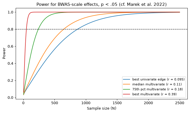
The best univariate effects need samples in the thousands, while multivariate effects of $r \approx 0.4$ are detectable with $N$ in the tens to low hundreds — roughly a 16–17-fold reduction (the variance-explained ratio $r^2$ is exactly 16-fold for 0.4 vs. 0.1), before any multiple comparisons correction (a multivariate model yields one test, so none is needed). Task-evoked multivariate patterns can be far stronger still ( $d > 3$ for some validated signatures), detectable in very small samples.

Wrap-up¶

Power depends on the effect size in the group analysis — the final common pathway for all design, acquisition, and analysis choices — and on the effective alpha after multiple comparisons correction.
Required samples grow explosively as effects shrink: $r = 0.5$ needs ~30 participants for one test; $r = 0.1$ needs ~780 — and several-fold more under correction. Two-group comparisons need ~4× the total sample of one-sample tests.
The minimum detectable effect size tells you what your planned N can honestly claim to test.
Post hoc effect sizes from significant voxels are inflated by selection — more so with small samples and strict thresholds — so base power analyses on unbiased, independent estimates.
Aggregating signal — a priori ROIs, networks, or multivariate patterns — trades voxel-level localization for dramatically larger effects, fewer tests, and higher power.