Chapter 27 Lab — Experimental Design and Task fMRI (Python) - Elements of fMRI Analysis

In this lab you will score fMRI designs before collecting any data. We follow a four-step arc:

Build the machinery: a canonical HRF and a design-matrix builder that turns event onsets into predicted BOLD regressors
Score competing designs: compute the efficiency of an A − B contrast for a blocked design, a dense fixed-ISI event-related design, and a sparse jittered event-related design
Diagnose collinearity with variance inflation factors (VIFs)
Map the detection–estimation tradeoff: score many designs under both a canonical-HRF model (contrast detection) and a flexible FIR model (HRF shape estimation)

Everything here uses simulated timing only — no scanner data required — which is exactly the point: efficiency depends purely on the design matrix, so you can (and should) evaluate designs before the study is run.

How to run this notebook. Run it in your browser from the tutorial site, in Google Colab, or in a local Jupyter environment with numpy, scipy, and matplotlib installed. See the chapter page for the concepts behind each step.

▶ This notebook is interactive. Click the ⏻ power icon at the top right of this page to run it in your browser — no installation needed (the kernel takes ~30–60 s to start the first time). Then run cells top to bottom, starting with the first code cell below: later cells depend on the imports and variables defined earlier, and will error if you skip ahead.

import numpy as np
import matplotlib.pyplot as plt
from scipy import stats

rng = np.random.default_rng(27)   # seeded RNG so event orderings are reproducible
np.set_printoptions(precision=3, suppress=True)
print("numpy", np.__version__)

numpy 2.4.6

Step 1 — The machinery: HRF and design builder¶

Task predictors are built by convolving a stimulus indicator function (1 during hypothesized neural activity, 0 elsewhere) with a canonical HRF (Chapter 18). All designs in this lab share:

run length $T = 480$ s, sampled at 1 s (480 “volumes”)
two event types, A and B, each lasting 2 s
event slots every 4 s (the minimum ISI); designs differ only in how slots are filled

The helper below returns a design matrix with columns [A, B, intercept].

T = 480                     # run length (s)
dt = 1.0                    # sampling resolution (s); think TR = 1
t = np.arange(0, T, dt)     # time grid for the run (one sample per second)
slots = np.arange(0, T, 4.0)          # candidate event onsets, every 4 s

def canonical_hrf(tt):
    # Double-gamma canonical HRF (SPM-style parameters), peak-normalized
    h = stats.gamma.pdf(tt, 6, scale=1) - stats.gamma.pdf(tt, 16, scale=1) / 6
    return h / h.max()

hrf = canonical_hrf(np.arange(0, 32, dt))   # sample the HRF over a 32-s window

def stimulus(onsets, dur=2.0):
    # Indicator function: 1 during events, 0 elsewhere
    s = np.zeros_like(t)
    for on in onsets:
        s[(t >= on) & (t < on + dur)] = 1.0
    return s

def design(onsets_A, onsets_B, dur=2.0):
    # Convolve each condition's indicator with the HRF; intercept last
    X = np.ones((len(t), 3))
    X[:, 0] = np.convolve(stimulus(onsets_A, dur), hrf)[:len(t)]
    X[:, 1] = np.convolve(stimulus(onsets_B, dur), hrf)[:len(t)]
    return X

fig, ax = plt.subplots(figsize=(6, 3))
ax.plot(np.arange(0, 32, dt), hrf, lw=2)
ax.axhline(0, color="gray", lw=0.5)
ax.set(xlabel="Time after neural event (s)", ylabel="Response (a.u.)",
       title="Canonical double-gamma HRF")
plt.tight_layout()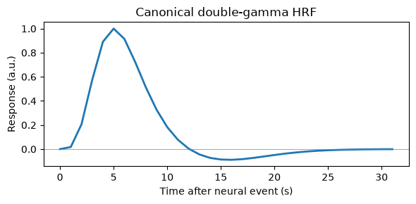

Step 2 — Three competing designs¶

We now fill the event slots three different ways, holding run length and conditions constant:

Blocked: 16-s blocks of A alternate with 16-s blocks of B (events presented back-to-back within each block, the classic A–B–A–B arrangement)
Dense fixed-ISI event-related: every slot holds an event, order randomized (60 A + 60 B, no rest)
Sparse jittered event-related: each slot is A, B, or rest with equal probability — the rest slots create variable, “jittered” inter-trial intervals

These are exactly the three arrangements in Figure 27.1 of the book.

# --- Blocked: alternating 16-s blocks (4 consecutive slots per block) ---
block_lab = np.tile(np.repeat([0, 1], 4), len(slots) // 8)   # AAAABBBB...
ons_block = (slots[block_lab == 0], slots[block_lab == 1])

# --- Dense fixed-ISI ER: every slot filled, random order, 50/50 A/B ---
dense_lab = rng.permutation(np.repeat([0, 1], len(slots) // 2))   # 60 A + 60 B, random order
ons_dense = (slots[dense_lab == 0], slots[dense_lab == 1])

# --- Sparse jittered ER: slots are A, B, or rest (1/3 each) ---
sparse_lab = rng.choice([0, 1, 2], size=len(slots), p=[1/3, 1/3, 1/3])   # 1/3 A, 1/3 B, 1/3 rest
ons_sparse = (slots[sparse_lab == 0], slots[sparse_lab == 1])

designs = {
    "Blocked (16 s)":  design(*ons_block),
    "Dense fixed-ISI": design(*ons_dense),
    "Sparse jittered": design(*ons_sparse),
}

fig, axes = plt.subplots(3, 1, figsize=(9, 6), sharex=True)
for ax, (name, X) in zip(axes, designs.items()):
    ax.plot(t, X[:, 0], color="tab:blue", lw=1.2, label="A")
    ax.plot(t, X[:, 1], color="tab:red", lw=1.2, label="B")
    ax.set_ylabel(name, fontsize=9)
    ax.set_yticks([])
axes[0].legend(loc="upper right", ncol=2, fontsize=8)
axes[-1].set_xlabel("Time (s)")
fig.suptitle("Predicted BOLD regressors for three arrangements of the same conditions")
plt.tight_layout()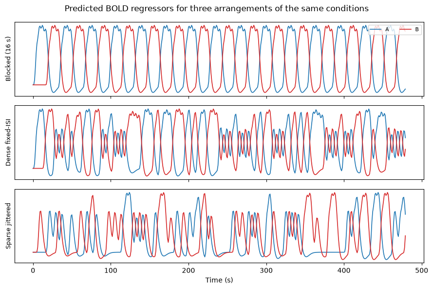

Note the qualitative differences: the blocked regressors swing slowly between high and low values (high variance, and A is high exactly when B is low); the dense regressors wiggle rapidly around a high plateau; the sparse regressors rise and fall as jitter lets the signal return toward baseline.

Score each design’s efficiency¶

The design-related variance of a contrast $c$ is $c\,(X^TX)^{-1}c^T$ , and efficiency is its inverse:

e_c = \frac{1}{c\,(X^TX)^{-1}\,c^T}

(1)

e_c — efficiency of contrast c · c — contrast vector (e.g., [1, −1, 0] for A − B) · X — design matrix (time × predictors)

where $c$ is the contrast vector, $X$ the design matrix, and the denominator $c\,(X^TX)^{-1}c^T$ the design-related variance of the contrast estimate.

We score two questions each design might be asked to answer:

A − B: which regions respond differently to the two conditions? ( $c = [1, -1, 0]$ )
A vs. baseline: which regions respond to A at all, relative to unmodeled rest? ( $c = [1, 0, 0]$ )

def contrast_efficiency(X, c):
    c = np.asarray(c, float)
    return 1.0 / (c @ np.linalg.pinv(X.T @ X) @ c)

c_diff = [1, -1, 0]      # A - B
c_base = [1, 0, 0]       # A vs. implicit baseline

print(f"{'design':<18}{'e(A - B)':>10}{'e(A vs baseline)':>18}")
for name, X in designs.items():
    print(f"{name:<18}{contrast_efficiency(X, c_diff):>10.1f}"
          f"{contrast_efficiency(X, c_base):>18.1f}")

fig, axes = plt.subplots(1, 2, figsize=(9, 3.2))
for ax, c, title in [(axes[0], c_diff, "Efficiency of [A - B] contrast"),
                     (axes[1], c_base, "Efficiency of [A vs. baseline]")]:
    vals = [contrast_efficiency(X, c) for X in designs.values()]
    ax.bar(range(3), vals, color="tab:blue")
    ax.set_xticks(range(3))
    ax.set_xticklabels(["Blocked", "Dense\nfixed-ISI", "Sparse\njittered"], fontsize=8)
    ax.set_title(title, fontsize=10)
    ax.set_ylabel("Efficiency (higher = better)", fontsize=8)
plt.tight_layout()

design              e(A - B)  e(A vs baseline)
Blocked (16 s)         750.9              22.2
Dense fixed-ISI        449.5              22.1
Sparse jittered        268.3             306.5

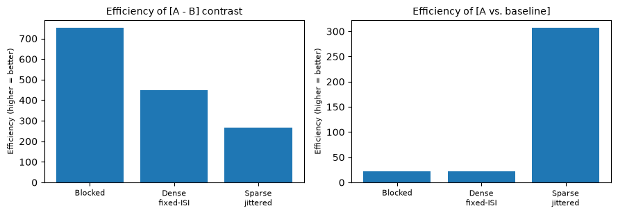
Interpretation. For the A − B contrast, the blocked design wins by a large margin — it concentrates the predicted A − B difference at a slow frequency with maximal variance, reproducing Figure 27.1B. The dense design does reasonably (randomized order still creates A − B variance), and the sparse design is least efficient because much of its time is spent at rest.

The picture changes for A vs. baseline. In the dense design, events occur constantly, so the A regressor hovers near a plateau and is partly confounded with the intercept — there is little “baseline” left to compare against. Jitter is what buys you peaks and valleys specific to each condition, so the sparse design holds its own for baseline comparisons despite having fewer trials. This is the core lesson: which design is best depends on which contrast you care about, and you should score the contrasts you actually plan to test.

Step 3 — Collinearity and variance inflation factors¶

Efficiency suffers when regressors are correlated — the model cannot decide which predictor deserves credit. Pairwise correlations miss the worst case, where one regressor is predictable from a combination of the others (including the intercept), so the standard diagnostic is the variance inflation factor:

\mathrm{VIF}_j = \frac{1}{1 - R_j^2}

(2)

VIFⱼ — variance inflation factor for regressor j · Rⱼ² — variance in regressor j explained by all the other predictors together

where $R_j^2$ is the proportion of variance in predictor $j$ explained by regressing it on all the other predictors.

VIF = 1 is perfect (orthogonal); ~2+ deserves attention; ~4–8+ is serious trouble.

We first compute VIFs for the three competing designs, then build the most common collinearity trap in real tasks: a cue event always followed by a stimulus event at a fixed short lag.

def vif(X):
    """VIF for each non-intercept column of X."""
    Xc = X[:, :-1] - X[:, :-1].mean(axis=0)   # drop intercept, center
    out = []
    for j in range(Xc.shape[1]):
        yj, Xo = Xc[:, j], np.delete(Xc, j, axis=1)
        b, *_ = np.linalg.lstsq(Xo, yj, rcond=None)
        out.append(np.sum(yj ** 2) / np.sum((yj - Xo @ b) ** 2))  # = 1/(1 - R^2)
    return np.array(out)

print("VIFs for the three competing designs (A shown; A and B are symmetric):")
for name, X in designs.items():
    r = np.corrcoef(X[:, 0], X[:, 1])[0, 1]
    print(f"  {name:<18} corr(A,B) = {r:6.2f}   VIF = {vif(X)[0]:6.2f}")

# The classic trap: a cue (A) always followed exactly 2 s later by a stimulus (B)
cue = ons_sparse[0]                                     # sparse design's A onsets
X_fixed = design(cue, cue + 2.0)                        # fixed 2-s cue-stim lag
X_jit = design(cue, cue + rng.choice([2.0, 6.0, 10.0], size=len(cue)))  # jittered 2/6/10-s lag

print()
for name, X in [("fixed 2-s lag ", X_fixed), ("jittered lag  ", X_jit)]:
    r = np.corrcoef(X[:, 0], X[:, 1])[0, 1]
    print(f"cue-stim, {name} corr(A,B) = {r:5.2f}   VIF = {vif(X)[0]:5.2f}   "
          f"e(A - B) = {contrast_efficiency(X, c_diff):6.1f}")

VIFs for the three competing designs (A shown; A and B are symmetric):
  Blocked (16 s)     corr(A,B) =  -0.99   VIF =  34.09
  Dense fixed-ISI    corr(A,B) =  -0.98   VIF =  20.61
  Sparse jittered    corr(A,B) =  -0.39   VIF =   1.18

cue-stim, fixed 2-s lag  corr(A,B) =  0.80   VIF =  2.84   e(A - B) =   35.1
cue-stim, jittered lag   corr(A,B) =  0.22   VIF =  1.05   e(A - B) =  128.1

Two different lessons here.

The no-rest trap. The blocked and dense designs have enormous VIFs (roughly 20–35): with no rest, an event is always on, so A + B is nearly constant and each regressor is almost perfectly (negatively) predictable from the other plus the intercept. Each individual $\hat{\beta}$ — “does A activate this region relative to baseline?” — is barely estimable, which is exactly why these designs scored so poorly on the A-vs-baseline contrast in Step 2. Yet the A − B contrast is estimated precisely: VIF is a per-parameter diagnostic, and specific contrasts can escape the collinearity. The sparse jittered design keeps VIFs near 1.

The fixed-lag trap. When a stimulus always follows its cue at the same short lag — a very natural way to program a task — the two convolved regressors correlate around 0.8, the VIF climbs toward the warning zone, and the efficiency of the A − B contrast collapses roughly four-fold. The model can barely tell cue-related from stimulus-related signal: true signal for one can masquerade as activation (or deactivation) of the other. Jittering the cue→stimulus interval decorrelates the regressors and restores efficiency — jitter is the cure.

Step 4 — The detection–estimation tradeoff¶

So far we assumed the canonical HRF is correct and asked how well designs detect contrasts. The complementary question is how well a design lets you estimate the shape of the response, using a finite impulse response (FIR) model with one free parameter per post-stimulus time point (here, 16 lags of 1 s per condition).

Both questions use the same efficiency formula with different design matrices:

Detection efficiency: $e_c$ for the A − B contrast under the canonical-HRF model
Estimation efficiency: $e = p \, / \, \mathrm{trace}[(X^TX)^{-1}]$ over the $p$ FIR parameters

We score many random designs that vary in their proportion of rest (jitter), plus the blocked design, on both criteria — a home-made version of Figure 27.4 in the book.

FIR_LAGS = 16      # estimate response at lags 0..15 s after onset

def fir_design(onsets_A, onsets_B):
    # One shifted-stick-function column per lag per condition; intercept last
    X = np.ones((len(t), 2 * FIR_LAGS + 1))
    for jcond, onsets in enumerate([onsets_A, onsets_B]):
        stick = np.zeros(len(t))
        stick[np.round(np.asarray(onsets) / dt).astype(int)] = 1.0
        for lag in range(FIR_LAGS):
            X[:, jcond * FIR_LAGS + lag] = np.roll(stick, lag)
            X[lag > np.arange(len(t)), jcond * FIR_LAGS + lag] = 0  # no wraparound
    return X

def estimation_efficiency(onsets_A, onsets_B):
    Xf = fir_design(onsets_A, onsets_B)
    v = np.diag(np.linalg.pinv(Xf.T @ Xf))[:-1]     # FIR columns only
    return (2 * FIR_LAGS) / v.sum()

def detection_efficiency(onsets_A, onsets_B):
    return contrast_efficiency(design(onsets_A, onsets_B), [1, -1, 0])

# Random event-related designs with varying amounts of rest (jitter)
rest_props = [0.0, 0.125, 0.25, 0.375, 0.5, 0.625]   # proportion of rest slots (jitter) to test
det, est, col = [], [], []
for p_rest in rest_props:
    for _ in range(8):                    # 8 random designs per rest level
        p_ev = (1 - p_rest) / 2           # split the non-rest slots evenly between A and B
        lab = rng.choice([0, 1, 2], size=len(slots), p=[p_ev, p_ev, p_rest])
        oA, oB = slots[lab == 0], slots[lab == 1]
        det.append(detection_efficiency(oA, oB))
        est.append(estimation_efficiency(oA, oB))
        col.append(p_rest)

det_block = detection_efficiency(*ons_block)
est_block = estimation_efficiency(*ons_block)

fig, ax = plt.subplots(figsize=(7, 5))
sc = ax.scatter(est, det, c=col, cmap="viridis", s=30)
ax.scatter([est_block], [det_block], marker="*", s=250, color="tab:orange",
           edgecolor="k", zorder=5, label="Blocked (16 s)")
ax.set(xlabel="HRF shape estimation efficiency (FIR model)",
       ylabel="Contrast detection efficiency (canonical HRF)",
       title="The detection-estimation tradeoff")
fig.colorbar(sc, label="Proportion of rest slots (jitter)")
ax.legend(loc="upper right")
plt.tight_layout()

print(f"Blocked design:  detection = {det_block:.1f},  estimation = {est_block:.3f}")
print(f"Best random ER:  detection = {max(det):.1f},  estimation = {max(est):.3f}")

Blocked design:  detection = 750.9,  estimation = 0.679
Best random ER:  detection = 498.7,  estimation = 22.875

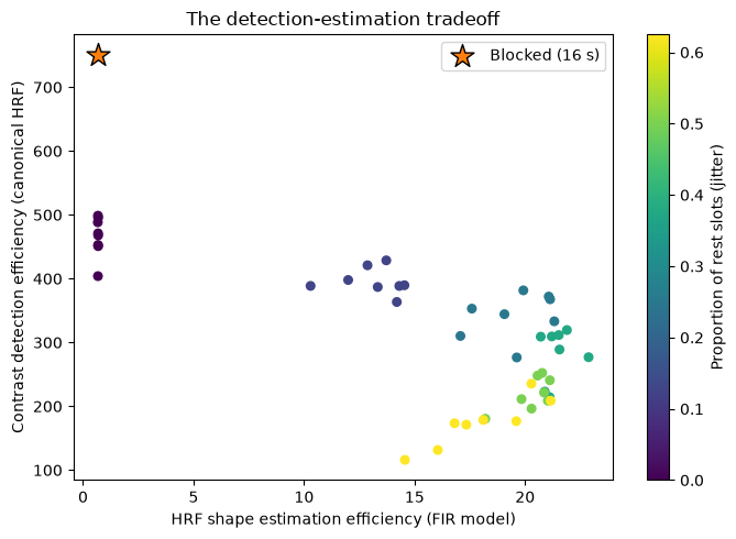
Interpretation. The blocked design (star) sits far up the detection axis but far left on estimation: its events are packed into predictable runs, so the shifted FIR sticks are nearly collinear and the response shape is almost unrecoverable. Random event-related designs form a cloud: adding jitter (lighter points) improves shape estimation — the varied spacing decorrelates the FIR columns — while trading away some detection efficiency. No design in the cloud dominates both axes: this is the tradeoff of Figure 27.4.

Where the book’s figure goes further is the frontier: m-sequences (pseudorandom sequences orthogonal to their own time-shifted copies) reach the estimation extreme, and genetic algorithms — which recombine pieces of the best designs across “generations,” using a fitness function that weights the contrasts and models you actually care about — find designs that beat random search on both axes and approach the theoretical limit. The CANlab OptimizeDesign toolbox (optimizeGA.m) implements such a GA for MATLAB, and the companion MATLAB live script for this chapter shows how to set one up.

Wrap-up and exercises¶

You scored designs before any data were collected using only $X$ : blocked designs win for contrast detection, jitter buys baseline comparisons and HRF estimation, VIFs flag collinearity, and detection versus estimation is a genuine tradeoff that optimization algorithms can navigate.

Try on your own:

Re-run Step 2 with 8-s and 32-s blocks. Where does the A − B efficiency peak, and why might very long blocks be risky in real data (hint: high-pass filters)?
In Step 4, add a fixed 4-s ISI, strictly alternating design (ABABAB...). Where does it land on the tradeoff plot, and why is its A − B detection efficiency so poor? (Hint: what temporal frequency does the A − B difference oscillate at, and what does the HRF do to high frequencies?)
Modify the efficiency scoring to include a high-pass filter: residualize the columns of $X$ against a discrete cosine basis (periods > 128 s) before computing $e$ . How much does the 16-s blocked design lose? What happens with 64-s blocks?
Write a mini-optimizer: generate 500 random designs at 30% rest and keep the one with the best weighted sum of detection and estimation efficiency (z-score each first). How much does the winner beat the average by?