Day 3 · Design, group inference, and ICA in practice

Day 3Session 3.4Kiehl1:00 hHands-on session

SPM results: group subjects, plotting, display, small-volume correction

In this hands-on session you run a second-level one-sample t-test in SPM12 on 50 subjects' auditory oddball contrast images, then use the Results interface to threshold, tabulate, plot and display group activations. It also covers masking, FWE versus uncorrected thresholds, extent thresholds, overlays on anatomy, and small volume correction for a priori regions.

Take-aways

  • A group one-sample t-test in SPM is a contrast of 1 on the intercept over subjects' contrast images.
  • Check the file order before adding covariates; SPM's file selector does not sort numerically.
  • Use FWE-corrected thresholds by default, and reserve small volume correction for regions specified before looking at the data.

Key terms

  • Specify 2nd-level
  • one-sample t-test
  • contrast manager
  • FWE correction
  • uncorrected threshold
  • extent threshold
  • maximum intensity projection (MIP)
  • sections and render overlays
  • small volume correction (SVC)
  • eigenvariate
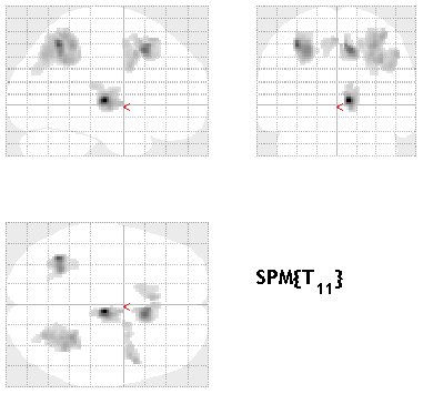
SPM-style glass brain showing thresholded t-statistics
SPM-style glass brain showing thresholded t-statistics. Lecture 3.3 slides (Wager)

Outline

What the session covers

01Second-level data and model setup

  • Data: 50 derivative-boosted contrast images per contrast (targets vs. standards, novels vs. standards) under 50subjects-stats.
  • The derivative boost adjusts HRF amplitude for latency; it is required to carry temporal or dispersion derivatives to the second level.
  • Specify 2nd-level creates a batch: choose an output directory, then select all 50 con images as scans.
  • MATLAB selects files in the order 1, 10, 11, ... 19, 2, 20; any covariate vector (e.g., age) must match this order.
  • Run the batch to write SPM.mat, then Estimate the model.

02Contrast manager

  • Results opens the contrast manager: design matrix on the right, defined contrasts on the left.
  • Choose t-contrast or F-contrast, Define new contrast, name it and enter weights (a single 1 for the group mean).
  • SPM accepts only estimable contrasts; valid contrasts are shown in green, invalid in red.
  • Select the contrast and press Done to proceed to masking and thresholding prompts.

03Masking and thresholding options

  • Apply masking: none, contrast or image; inclusive masks keep voxels significant in the mask contrast, exclusive removes them.
  • Masking at p = 0.05 uncorrected (default) does not change the target contrast's p-values, only which voxels are shown.
  • p-value adjustment: FWE at 0.05 means one map in twenty contains a false positive anywhere; none gives uncorrected voxel-level p, default 0.001.
  • Uncorrected p = 0.001 over 50,000 voxels gives about 50 expected false positives.
  • Extent threshold k shows only clusters with at least k voxels; the default 0 allows single-voxel activations.

04Glass brain, tables and files

  • The Graphics window shows a maximum intensity projection (MIP) on a glass brain in three orthogonal planes.
  • The MIP is surfable: drag the red cursor or right-click for a menu; the design matrix with the selected contrast is shown alongside.
  • Whole brain lists clusters and maxima more than 8 mm apart with peak-, cluster- and set-level p-values; current cluster lists maxima 4 mm apart.
  • Clicking a row in the table moves the cursor; coordinates can also be typed in the Interactive window.
  • con_000n.nii and spmT_000n.nii images are written to the analysis directory; Save writes the thresholded map as NIfTI.

05Plotting and overlays

  • Plot offers contrast estimates with 90 percent CI, fitted responses, event-related responses, parametric responses and Volterra kernels.
  • Event-related options include fitted response with PSTH, with 90 percent CI, or with adjusted data; use hold to compare conditions.
  • Typing Y in MATLAB returns fitted values and y the adjusted data (adjusted for confounds and filtering).
  • Overlays: slices (three adjacent transaxial slices), sections (three intersecting surfable planes) or render on a surface.
  • For render, choose a subject rendering or the canonical mesh cortex_20484.surf.gii in the SPM canonical folder.

06Small volume correction and data extraction

  • With an a priori anatomical hypothesis, press small volume in the Interactive window and define a sphere, box or mask image.
  • Example from the manual: a 30 mm sphere centered at 44 16 0 for Broca's area.
  • The search volume shrinks and corrected p-values become more significant than whole-brain correction.
  • The eigenvariate button extracts a region's first eigenvariate (VOI_name.mat), a weighted mean robust to heterogeneous voxels.
Five dynamic connectivity states rendered on cortical surfaces — Rashid et al. (2014), Frontiers in Human Neuroscience

Hands-on

Step by step

The walk-through below is distilled from the course cheat sheets. Data paths refer to the course Dropbox folder (e.g. data/auditory_oddball).

  1. Click Specify 2nd-level; set the output directory to ../mind/data/auditory_oddball/50subjects-stats/Group-stats-targets_vs_standards.
  2. Under Scans, select all 50 files 1-db_targets_vs_standards.img ... 50-db_targets_vs_standards.img from 50_subs_contrast_images_target_stimuli and click Done.
  3. Note the selection order (1, 10, 11, ..., 2, 20, ...); any covariate vector must match it. Click the green arrow to build SPM.mat.
  4. Click Estimate, select the new SPM.mat, and run.
  5. Click Results, select SPM.mat, Define new contrast named target vs standard with weight 1, submit, OK, Done.
  6. Answer the prompts: masking none, p-value adjustment FWE, p = 0.05, extent threshold 0.
  7. Inspect the glass-brain MIP; press whole brain and current cluster for results tables; click rows to move the cursor.
  8. Press Plot: Contrast estimates and 90% CI, then Fitted responses; type Y or y in MATLAB to inspect the values.
  9. Use Overlays: sections (select a normalized structural or SPM canonical image) and render (cortex_20484.surf.gii).
  10. Re-threshold with none at p = 0.001 and an extent threshold (e.g., 10 voxels) and compare to the FWE map.
  11. Press small volume, define a sphere around an a priori coordinate, and compare corrected p-values with the whole-brain table.
  12. Repeat the steps for the novels vs. standards contrast images.
Cheat sheet: second-level t-test — full cheat sheet

Mind fMRI Image Acquisition and Analyses Course - Cheat Sheet for Second Level (one sample t-test).

We have prepared 50 subjects worth of data for this exercise.

Two different contrasts have been included. Targets vs standards and Novels vs standards.

These data are located in ../mind/data/auditory_oddball/50subjects-stats/50_subs_contrast_images_target_stimuli

These data are located in ../mind/data/auditory_oddball/50subjects-stats/50_subs_contrast_images_target_stimuli

Each of these directories contains 50 derivative boosted contrast images. Recall that the derivative boost adjusts the amplitude of the HRF to address latency effects. See the Calhoun et al paper. Importantly, the derivative boost is necessary if you want to utilize the temporal (and/or dispersion) components from the first level into the second level analyses.

To start off second level (group) analyses, click on the spm button ‘Specify 2nd level’. This will pull up a batch GUI. The batch GUI first requires you to specify a directory to place the statistics files in. So select:

From here ../mind/data/auditory_oddball/50subjects-stats/ select

“Group-stats-targets_vs_standards”

The next data that needs to be entered are the contrast scans for analyses. Highlight/click on ‘scans’ and then go down to ‘specify’. Go to the directory: ../mind/data/auditory_oddball/50subjects-stats/50_subs_contrast_images_target_stimuli and right click and select ALL the images.

1-db_targets_vs_standards.img

2-db_targets_vs_standards.img

……

50-db_targets_vs_standards.img

Please note the ordering of the images in the matlab GUI – you will see that it selects them 1, 10, 11, 12, 13, 14, 15, 16, 17, 18, 19, 2, 20, 21……. This is not from 1-50……so this is ok, but if you enter any covariates (i.e., age) then your vector of age data MUST match up to the order of these images…….(this ordering was done on purpose to highlight this common problem).

Click ‘done’ once the images are selected.
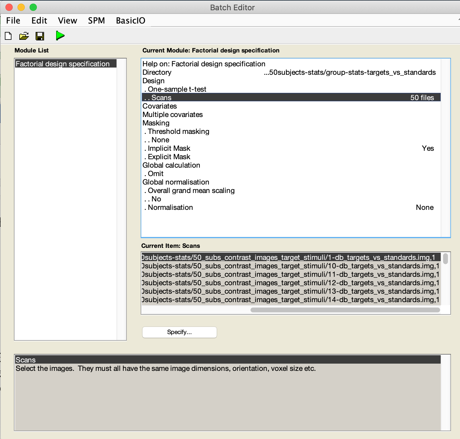
Graphical user interface, text, application Description automatically generated

Click on the green arrow and this will compute the design matrix and create an SPM.mat file.

Now click ‘estimate’ button in spm. Select the SPM.mat in the “Group-stats-targets_vs_standards” directory.

The green arrow will illuminate. Click it to run this model.

Now you may review the results.

Click on ‘Results’. Select the SPM.mat file above.

The contrast manager will come up. Define new contrast. Specify a name ‘target vs standard’. Enter a contrast value of ‘1’. Click submit, then click ok. Then click done.

Estimate the contrast and then complete the subsequent steps (no masking, FWE, p < .05) (thresholding at p < .05 FWE Corrected) and this will display the group results. You may then play around with the display/plot routines to interrogate the data.

Repeat the steps above if you want analyze the novel stimuli.

From the instructors' research

Related figures

Examples of these concepts in published work by the course instructors.

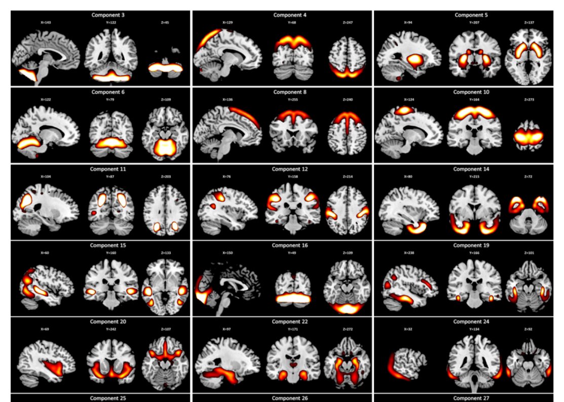
Source-based morphometry gray matter components predicting recidivism
Source-based morphometry gray matter components predicting recidivism. Kiehl et al. (2018), NeuroImage: Clinical
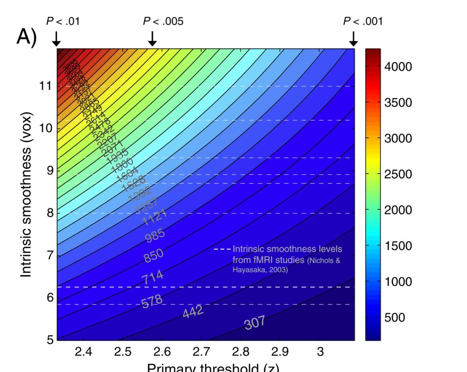
Cluster extent thresholds versus smoothness and primary threshold
Cluster extent thresholds versus smoothness and primary threshold. Woo et al. (2014), NeuroImage