Day 3 · Design, group inference, and ICA in practice

Day 3Session 3.6Calhoun, Kiehl1:30 hHands-on session

ICA of fMRI: implementation

In this hands-on session you run a group ICA in the GIFT toolbox, following the GIFT walkthrough, on the course's auditory oddball data. You set up the analysis parameters, run the data reduction, ICA, back-reconstruction and group statistics steps, and then use the display and sorting tools to identify task-related components.

Take-aways

  • A GIFT analysis is a sequence of setup, reduction, ICA, back-reconstruction, calibration and group statistics that can be resumed step by step.
  • The key choices are number of components, preprocessing and scaling, PCA type and back-reconstruction method.
  • Components are identified by viewing maps and time courses and by sorting against the task model or spatial templates.

Key terms

  • GIFT
  • Setup ICA
  • prefix
  • MDL component estimation
  • Infomax
  • ICASSO
  • data reduction (PCA)
  • back-reconstruction
  • Component Explorer
  • temporal sorting
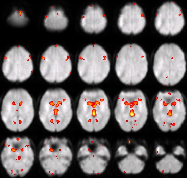
Spatial ICA component maps on grey axial slices (GIFT output)
Spatial ICA component maps on grey axial slices (GIFT output). Lecture 3.5 slides (Calhoun)

Outline

What the session covers

01Setup ICA: main parameters

  • Start GIFT (gift.m adds paths), click Setup ICA and choose an output directory; all outputs share a user-entered prefix.
  • Select the fMRI data files; a Subject.mat file records subjects, sessions and files.
  • Optionally estimate the number of components with the MDL criterion; otherwise enter Number of IC (default 20).
  • Auto-fill data reduction sets first-step PCs to 1.5 times the number of final components when two reduction steps are used.
  • Algorithms include Infomax (default), FastICA, ERICA, JADE, Constrained ICA and GIG-ICA; ICASSO or MST runs ICA repeatedly for stability.
  • Choose serial or parallel execution.
02Setup ICA defaults: preprocessing, PCA and scaling

  • Pre-processing options: remove mean per timepoint, remove mean per voxel, intensity normalization (mean 100) or variance normalization (z-scores).
  • Mask: default mask from the mean of each subject's first file, or a user-supplied Analyze/NIfTI mask.
  • PCA types: standard, expectation maximization, SVD, MPOWIT and STP; stack datasets in single precision when memory allows.
  • Group PCA can be subject-specific or grand mean; up to two reduction steps, with Number of PC (Step 1) per subject.
  • Back-reconstruction: regular (GICA2), spatial-temporal regression, GICA3 or GICA; GICA3 preserves both the aggregate map and the data.
  • Scaling: none, percent signal change, z-scores, scaling in time courses, or in maps and time courses; spatial ICA is the default.
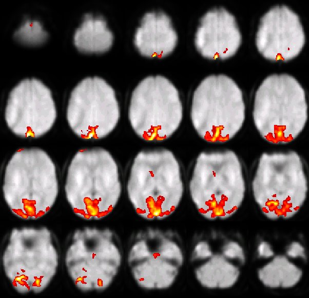
Group ICA component map displayed on axial slices
Group ICA component map displayed on axial slices. Lecture 3.5 slides (Calhoun)

03Run analysis

  • Run Analysis takes the *ica_parameter_info.mat file and offers All, Resume or individual steps.
  • Steps: parameter initialization, data reduction, calculate ICA, back reconstruction, calibrating components, group stats.
  • Group stats writes mean, standard deviation and t-statistic maps and time courses per session in Analyze/NIfTI.
  • Command line: load the parameter file and call icatb_runAnalysis(sesInfo, step) with steps 1 to 8.
  • Progress and settings are logged to the _results.log file; Analysis Info summarizes parameters and output files.

04Display tools

  • Display GUI combines Component Explorer, Subject Component Explorer, Orthogonal Viewer and Composite Viewer.
  • Display Defaults control image values (positive, negative, absolute), z-score conversion, threshold, anatomical plane, slice range and images per figure.
  • Component Explorer shows all components of a viewing set (e.g., mean of all subjects) with time courses; page through to find task-related components.
  • Subject Component Explorer shows one component across all subjects and sessions.
  • Orthogonal Viewer compares the BOLD time course at a clicked voxel with the ICA time course and lists the top five components.
  • Composite Viewer overlays up to five components on an anatomical image such as ch2bet.nii.

05Sorting components

  • Temporal sorting compares ICA time courses with SPM model regressors using correlation, kurtosis or multiple linear regression (R-squared).
  • Select the SPM design matrix under Display GUI Options; regressors like target*bf(1) define the model time courses.
  • Results are written to files with suffix regression.txt and partial_corr.txt.
  • The enlarged time-course plot offers power spectrum, split time courses, event average and Adjust ICA to remove other regressors' variance.
  • Spatial sorting uses templates in icatb_templates with multiple regression, correlation, kurtosis or maximum voxel criteria.
Resting-state networks matched to BrainMap task networks — Lecture 3.5 slides (Calhoun)

Hands-on

Step by step

The walk-through below is distilled from the course cheat sheets. Data paths refer to the course Dropbox folder (e.g. data/auditory_oddball).

  1. Add GIFT to the MATLAB path (run gift.m) and open the GIFT toolbox window.
  2. Click Setup ICA, choose an output directory (e.g., ../mind/data/auditory_oddball_ica) and enter a prefix such as Aod.
  3. Click Select to choose the preprocessed auditory oddball fMRI files for each subject; confirm the Subject.mat summary.
  4. Set Number of IC to 20 (or estimate with MDL), keep auto-fill data reduction, algorithm Infomax, analysis type Regular (or ICASSO).
  5. In Setup ICA Defaults check preprocessing (e.g., remove mean per timepoint), default mask, standard PCA, two reduction steps, GICA3 back-reconstruction and z-score scaling; press Done and accept ICA options.
  6. Click Run Analysis, select Aod_ica_parameter_info.mat, choose All and wait for data reduction, ICA, back-reconstruction, calibration and group stats.
  7. Click Analysis Info to review parameters and output files; check the _results.log file.
  8. In Display GUI choose Component Explorer with viewing set mean for all subjects and sessions; page through Aod_mean_component_ica_s_all_0xx images to find task-related components.
  9. Use Subject Component Explorer for a chosen component to examine consistency across subjects.
  10. Open Orthogonal Viewer, click a voxel in auditory cortex and compare the BOLD and ICA time courses.
  11. Enable Sort Components with temporal sorting, Multiple Regression, select the SPM design matrix and target/novel regressors; view the R-squared ordering.
  12. In the enlarged time-course window use Event Average for the target regressor, then overlay the top components in the Composite Viewer on ch2bet.nii.

GIFT walk-through (PDF)

GIFT documentation

From the instructors' research

Related figures

Examples of these concepts in published work by the course instructors.

Simulated spatial component map for group ICA
Simulated spatial component map for group ICA. Allen et al. (2012), NeuroImage
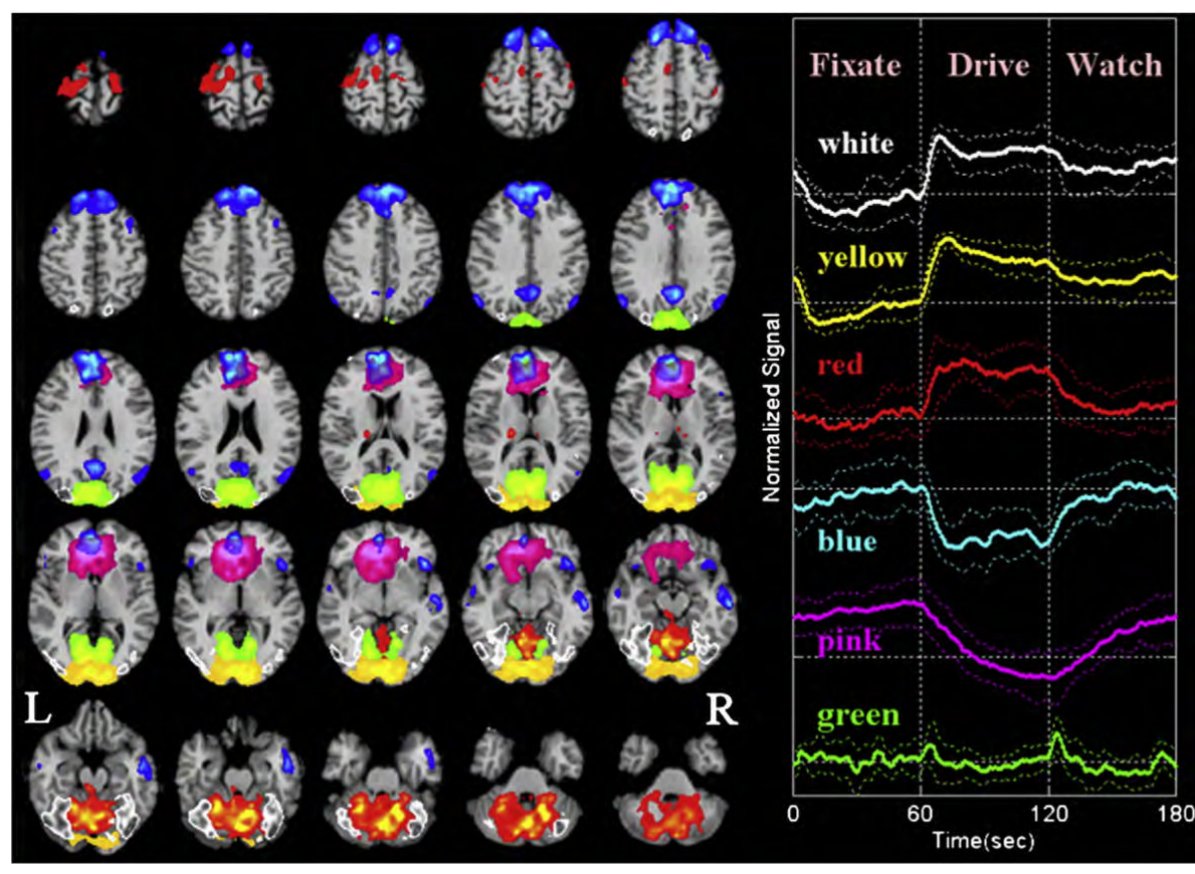
Multiple networks identified during simulated driving
Multiple networks identified during simulated driving. Calhoun et al. (2009), NeuroImage