Multivariate Decomposition: PCA and ICA
Run this code: ⚡ In-browser lab · Colab · MATLAB Online
Overview
Everything up to this point in the book has been largely univariate: a model is fit to one voxel at a time, and the results are stitched into maps. Multivariate decomposition methods flip this around. They operate on many variables at once — typically the full matrix of one subject’s fMRI data, with time points as rows and voxels as columns — and factor it into a small number of components, each pairing a spatial map (a pattern over voxels) with a time course. The components are latent variables: not directly measured, but expressed across many measured voxels. Decomposition methods are workhorses of functional connectivity analysis, and ICA in particular is the most widely used method for identifying resting-state networks. The broader family includes factor analysis, multidimensional scaling, and non-negative matrix factorization — the members differ mainly in the constraints they impose (orthogonality vs. independence), whether they model noise explicitly, and how they normalize the data — but PCA and ICA are the bedrock, and the focus here.
Principal components analysis reduces the dimensionality of a set of correlated variables while retaining as much variance as possible. It transforms the original variables into new ones — the principal components — that are uncorrelated and ordered by the variance they explain. Formally, PCA eigen-decomposes the data covariance (or correlation) matrix, , where the columns of are eigenvectors defining linear combinations of voxels and the diagonal of holds eigenvalues proportional to each component’s share of variance. In practice the components are computed via the singular value decomposition of the mean-centered data:
X — mean-centered data (time × voxels) · U — component time courses in columns (T × T, orthonormal) · S — diagonal matrix of singular values, sorted largest to smallest · Vᵀ — eigenimages (spatial maps) in rows (V × V orthonormal)
where is the mean-centered data matrix, () and () are orthonormal matrices, and is diagonal with singular values sorted largest to smallest.
In fMRI terms, each column of is an eigenimage — a spatial mode capturing covariance structure across voxels — and the corresponding column of (scaled by its singular value) is that eigenimage’s time course. The data are exactly the sum of rank-one layers, — where and are the th columns of and and the th singular value — and truncating the sum after terms gives the best possible rank- reconstruction. The proportion of variance explained by component is , its squared singular value as a share of the total.
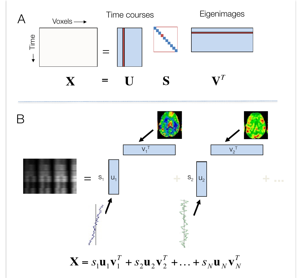
Overview of PCA via the singular value decomposition. (A) The time voxels data matrix is factored as : holds the eigenimages (spatial maps), their associated time courses, and the singular values. (B) Equivalently, is a sum of rank-one components , each the outer product of a time course and a spatial map, weighted by its singular value. (Figure 31.1 from the book. © the authors and MIT Press; reproduced with permission — not covered by this site’s CC-BY license.)
Because components are ordered, later ones can often be discarded with little loss, making PCA a natural data-reduction and exploration tool — for spotting outlier volumes in quality control, for finding distributed patterns related to tasks, and as a preprocessing step for ICA and for the predictive models of Part 7. Common rules for choosing how many components to keep: look for an “elbow” where the scree plot of variance explained decelerates; retain enough components to explain a target proportion of variance (e.g., 90%); keep components with eigenvalues greater than 1 (more than one original variable’s worth); or compare against decompositions of permuted (randomized) data and keep components that beat chance.
PCA’s guarantees come with a catch: the components must be orthogonal, and they chase variance. Real signal sources — brain networks, physiological artifacts, scanner drift — have no obligation to be orthogonal to one another or to line up with directions of maximal variance. When two sources overlap or correlate, the first PC typically captures a variance-weighted blend of both and later PCs capture orthogonal remainders: the subspace is right, but the axes within it are rotated away from the true sources. Independent components analysis addresses exactly this. It models the data as a linear mixture of latent sources,
X — data (time × voxels, T × V) · A — mixing matrix (T × k), component time courses in columns · S — source matrix (k × V), spatially independent maps in rows · k — number of components
where is the data, the mixing matrix () holds each component’s time course in its columns, the source matrix () holds spatially independent maps in its rows, and is the number of components.
Neither nor is observed; ICA seeks an unmixing matrix such that recovers the sources — blindly, without knowing the mixing process.
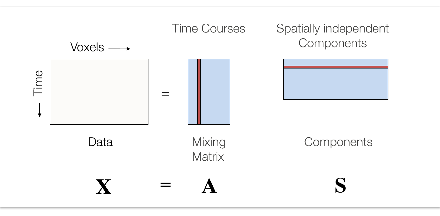
Overview of spatial ICA. The time voxels data is modeled as a mixing matrix — whose columns are component time courses — times a source matrix whose rows are statistically independent spatial maps. (Figure 31.2 from the book. © the authors and MIT Press; reproduced with permission — not covered by this site’s CC-BY license.)
What makes this possible is a stronger criterion than PCA’s: statistical independence, — where and are any two component sources and denotes a probability density — based on higher-order properties of the distributions rather than just second moments. Independence implies uncorrelatedness, but the converse holds only for Gaussian signals — uncorrelated non-Gaussian signals can still carry higher-order dependence. ICA exploits two facts: many real-world signals are non-Gaussian, and by the Central Limit Theorem, mixing non-Gaussian signals pushes the mixtures toward Gaussianity. So ICA searches for the unmixing that makes the recovered components as non-Gaussian as possible — via algorithms such as infomax (maximizing entropy) or FastICA and JADE (working on kurtosis and related contrasts). At least of the sources must be non-Gaussian; with multiple Gaussian sources the model is identifiable only up to an orthogonal rotation. The flexibility carries costs: components have arbitrary sign, scale, and order, and are not ranked by importance, so researchers must inspect and label them. In fMRI, the standard variant is spatial ICA — maximizing independence of the spatial maps, consistent with the idea that different networks involve distinct sets of voxels — rather than temporal ICA, since tasks and artifacts routinely induce correlated time courses. Before ICA, data are typically mean-centered, whitened, and reduced with PCA. Calling ICA components “networks” is something of a misnomer — nothing guarantees that regions loading on a component are interconnected — but the usage is standard, and ICA-derived resting-state networks replicate remarkably well across subjects and sessions. ICA is also widely used for denoising during preprocessing.
In practice ICA is usually run on a group of subjects. The most common approach is temporal concatenation: stack each of the subjects’ matrices into an matrix , and fit , so all subjects share one set of group spatial maps while each subject’s block of () provides subject-specific time courses. Subject-specific maps are then recovered by back-reconstruction: either invert the model per subject (solve for ), or use the two-stage dual regression. In stage 1 (spatial regression), each subject’s data are regressed onto the group maps, yielding a time course per component — each map’s expression at every time point, controlling for the other maps. In stage 2 (temporal regression), the same subject’s data are regressed onto those time courses, yielding subject-specific spatial maps. Group inference follows naturally: t-tests on the subject-level maps identify voxels reliably loading on each component, and the subject-level time courses can serve as dependent variables in GLMs relating components to tasks and behavior. Because ICA solutions can vary across studies (noise sensitivity; sign and scale ambiguity), a popular strategy is to run dual regression against fixed, labeled template networks from large-scale resting-state studies — trading within-subject independence for comparability — while newer approaches such as Group Information-guided ICA and the NeuroMark pipeline estimate subject-level components constrained to match high-quality group templates. Popular implementations include MELODIC (FSL) and the GIFT toolbox (MATLAB).
Hands-on tutorial
The best way to understand what PCA and ICA each can and cannot do is to build data where the truth is known. We simulate two source “networks” — each a spatial map paired with a time course — mix them into a time voxels matrix with noise, and then ask each method to recover them. The key manipulation: the two spatial maps overlap, so the true sources are not orthogonal — though, being sparse blocks, they remain close to statistically independent. The labs then push further: scree plots for dimensionality, and a miniature dual regression on a simulated “group.”
Step 1 — Simulate mixed sources. Two spatial maps (overlapping blocks of voxels) and two event-driven time courses combine as .
% Requires CanlabCore + SPM12 on your MATLAB path
% Adapted from CANlab tutorials (github.com/canlab)
rng(7);                                        % seed for reproducibility
T = 200; V = 360; TR = 2;                      % T = time points, V = voxels, TR = repetition time (s)

% Two overlapping spatial maps (non-orthogonal sources)
s1 = zeros(1, V); s1(1:150)  = 1;              % "network" 1: voxels 1-150
s2 = zeros(1, V); s2(91:255) = 1;              % "network" 2: voxels 91-255 (overlap!)
S_true = [s1; s2];                             % k x V source-map matrix

% Two event-related time courses via the canonical HRF
a1 = onsets2fmridesign({[20 100 180 260 340]'}, TR, T*TR);   % network-1 event onsets (s)
a2 = onsets2fmridesign({[60 140 220 300 380]'}, TR, T*TR);   % network-2 event onsets (s)
A_true = [a1(:,1) a2(:,1)];                    % T x k: HRF-convolved regressors (drop intercept column)

X = A_true * S_true + 0.3 * randn(T, V);       % mix + Gaussian noise (SD = 0.3)
s1 * s2' / (norm(s1) * norm(s2))               % cosine ~0.4: maps not orthogonal
import numpy as np
from scipy.stats import gamma
rng = np.random.default_rng(7) # seed for reproducibility
T, V, TR = 200, 360, 2.0 # T = time points, V = voxels, TR = repetition time (s)
# Two overlapping spatial maps (non-orthogonal sources)
s1 = np.zeros(V); s1[0:150] = 1 # "network" 1: voxels 1-150
s2 = np.zeros(V); s2[90:255] = 1 # "network" 2: voxels 91-255 (overlap!)
S_true = np.vstack([s1, s2]) # k x V source-map matrix
# Two event-related time courses via a double-gamma HRF
t = np.arange(0, 32, TR) # HRF support: 0-32 s, sampled every TR
hrf = gamma.pdf(t, 6) - gamma.pdf(t, 16) / 6 # peak (~6 s) minus undershoot (~16 s)
hrf = hrf / hrf.max() # normalize to peak 1 -> signal has ~unit amplitude
def timecourse(onsets_s):
stick = np.zeros(T); stick[(np.array(onsets_s) / TR).astype(int)] = 1
return np.convolve(stick, hrf)[:T]
A_true = np.column_stack([timecourse([20, 100, 180, 260, 340]), # network-1 event onsets (s)
timecourse([60, 140, 220, 300, 380])]) # network-2 event onsets (s)
X = A_true @ S_true + 0.3 * rng.standard_normal((T, V)) # mix + Gaussian noise (SD = 0.3)
cos = s1 @ s2 / (np.linalg.norm(s1) * np.linalg.norm(s2))
print(f"cosine(map 1, map 2) = {cos:.2f}")
# cosine ~0.4: the maps overlap, so they are not orthogonalExample output: the two “network” maps are far from orthogonal — their cosine similarity is well above 0:
cosine(map 1, map 2) = 0.38Step 2 — PCA mixes, ICA unmixes. PCA (via SVD) captures the right two-dimensional subspace — the scree plot shows two components towering over the noise floor — but its orthogonal axes are rotated blends of the two correlated sources. FastICA, run on the same two-dimensional reduction, recovers maps that match the true sources almost perfectly.
% PCA via SVD of the mean-centered data
Xc = X - mean(X);                              % mean-center each voxel's time series
[U, Ssv, Vsv] = svd(Xc, 'econ');               % economy SVD: Xc = U * Ssv * Vsv'
var_explained = 100 * diag(Ssv).^2 / sum(diag(Ssv).^2);   % squared singular values -> % variance
figure; plot(var_explained(1:10), 'ko-'); title('Scree plot');   % first 10 components

pc_maps = Vsv(:, 1:2)';                        % eigenimages (rows)
disp('|corr| between true sources and PCA maps:')
disp(abs(corr(S_true', pc_maps')))             % PCs blend the sources

% Spatial ICA: the full lab implements FastICA from scratch in ~15 lines;
% with GIFT installed use icatb_fastICA, or CanlabCore's ica() on fmri_data
from sklearn.decomposition import FastICA
# PCA via SVD of the mean-centered data
Xc = X - X.mean(axis=0) # mean-center each voxel's time series
U, sv, Vt = np.linalg.svd(Xc, full_matrices=False) # economy SVD: Xc = U @ diag(sv) @ Vt
var_explained = 100 * sv**2 / np.sum(sv**2) # squared singular values -> % variance
print("Variance explained by PCs 1-4:", var_explained[:4].round(1))
import matplotlib.pyplot as plt
plt.plot(np.arange(1, 11), var_explained[:10], 'ko-') # scree plot: first 10 components
plt.xlabel('component'); plt.ylabel('% variance explained'); plt.title('Scree plot')
pc_maps = Vt[:2] # eigenimages (first 2 rows of V^T)
print("|corr| true sources vs PCA maps:")
print(np.abs(np.corrcoef(S_true, pc_maps)[:2, 2:]).round(2)) # blended
# Spatial ICA: voxels are the samples, so decompose the transpose
ica = FastICA(n_components=2, # k = 2 components (chosen from the scree plot)
random_state=0, # fixed seed: ICA results vary by initialization
whiten="unit-variance") # whitening = the PCA pre-reduction step
ic_maps = ica.fit_transform(Xc.T).T # k x V independent spatial maps
ic_time = ica.mixing_ # T x k component time courses
print("|corr| true sources vs ICA maps:")
print(np.abs(np.corrcoef(S_true, ic_maps)[:2, 2:]).round(2)) # ~1.0Example output: two components tower over a flat noise floor in the scree plot, and the correlation matrices tell the story — each PC mixes both sources, while each IC matches exactly one:
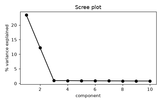
Scree plot of the simulated data: components 1 and 2 stand far above the flat noise floor, and an elbow appears at component 3. The MATLAB tab’s plot is analogous.
Variance explained by PCs 1-4: [23.4 12.2  1.   1. ]
|corr| true sources vs PCA maps:
[[0.58 0.78]
 [0.73 0.68]]
|corr| true sources vs ICA maps:
[[0.98 0.05]
 [0.05 0.98]]
You should see PCA map–source correlations well below 1 (each PC correlates with both sources), while each ICA map correlates near 1.0 with exactly one source. Same subspace, different axes — the independence criterion is what points the axes at the sources. The full labs complete the arc: reconstructing from rank-one layers, the scree/permutation view of dimensionality, and a mini dual regression that recovers subject-specific time courses and maps from a concatenated “group” dataset.
Open the full Python lab notebook → or download the MATLAB live script, which mirrors it using CANlab tools.


Thought questions
PCA components are orthogonal and variance-ranked; ICA components are independent, unordered, and of arbitrary sign and scale. For each property, give a concrete fMRI scenario where it is an asset and one where it is a liability.
Spatial ICA assumes networks are spatially independent, yet the chapter notes that regions loading on one component need not be interconnected, and overlapping “hub” regions belong to multiple networks. How would violations of spatial independence distort the recovered maps, and what might temporal ICA recover instead in the same data?
ICA works because mixtures of non-Gaussian sources are more Gaussian than the sources themselves. What kinds of fMRI signals and artifacts are strongly non-Gaussian, and what would happen to an ICA decomposition if the dominant sources of variance were nearly Gaussian?
A lab runs group ICA on its own 30-subject study; another performs dual regression against published template networks from a 1,000-subject consortium. Compare the two strategies for (a) sensitivity to this sample’s idiosyncratic networks, (b) replicability across studies, and (c) interpretability of a patient-vs-control difference on “the default mode network.”
Choosing the model order changes what ICA finds: small merges networks, large splits them into subnetworks. Is there a “true” number of brain networks? Defend a strategy for choosing and reporting in a study linking network expression to a clinical variable.
Quiz yourself
Q1. In a decomposition of a time voxels fMRI matrix, what two things does each component pair together?
Answer: A spatial map (a pattern of weights over voxels — an eigenimage in PCA, an independent map in ICA) and an associated time course describing how strongly that pattern is expressed at each time point.
Q2. In the SVD of mean-centered fMRI data, where are the eigenimages, their time courses, and the variance information?
Answer: The columns of (rows of ) are the eigenimages; the columns of hold the corresponding time courses; and the diagonal of holds the singular values, whose squares (divided by their sum) give each component’s proportion of variance explained.
Q3. Name three common rules for deciding how many principal components to retain.
Answer: Look for an elbow (deceleration) in the scree plot of variance explained; keep enough components to reach a variance threshold such as 90%; keep components with eigenvalues > 1; or use permutation testing to keep components explaining more variance than in randomized data. (Any three.)
Q4. Why is statistical independence a stronger requirement than uncorrelatedness, and for what kind of signals are the two equivalent?
Answer: Independence requires the joint distribution to factorize, , constraining all higher-order moments, whereas uncorrelatedness only constrains second moments. The two coincide only for Gaussian signals — uncorrelated non-Gaussian signals can still have higher-order dependence, which is exactly what ICA exploits.
Q5. In the ICA model for fMRI, what do and contain, and what does ICA actually estimate?
Answer: (the mixing matrix) contains each component’s time course in its columns; (the source matrix) contains spatially independent maps in its rows. Neither is observed: ICA estimates an unmixing matrix such that approximates the sources, without knowledge of the mixing process.
Q6. Why can ICA fail if more than one source is Gaussian?
Answer: Any orthogonal rotation of jointly Gaussian variables has exactly the same distribution, so with multiple Gaussian sources the unmixing matrix is only identifiable up to an orthogonal transformation — there is no unique independent solution to find.
Q7. Why is spatial ICA preferred over temporal ICA for fMRI?
Answer: Spatial ICA matches the assumption that different brain networks engage largely distinct sets of voxels (independent spatial maps), while temporal independence is less plausible — tasks and artifacts routinely produce correlated time courses across components. Spatial ICA also suits fMRI’s many-voxels, fewer-time-points geometry.
Q8. Describe the two stages of dual regression and what each produces.
Answer: Stage 1 (spatial regression): regress each subject’s data onto the group spatial maps, yielding a subject-specific time course per component, controlling for the other maps. Stage 2 (temporal regression): regress the same subject’s data onto those time courses, yielding subject-specific spatial maps. The time courses and maps then support group-level tests relating components to tasks, behavior, or group status.
 The book: Elements of Functional Magnetic Resonance Imaging — Wager & Lindquist, MIT Press