Network Analysis
Run this code: ⚡ In-browser lab · Colab · MATLAB Online
Overview
Network analysis represents the brain as a set of interconnected nodes (brain regions or voxels) and edges (anatomical or functional connections), letting us study brain organization, network properties, and dynamics with the mathematical machinery of graph theory — a field whose roots reach back to Euler in the mid-1700s. In network neuroscience, functional connectomes are used to estimate network topology and higher-order graph-theoretic properties: global properties like efficiency and small-worldness, sub-network structure (“communities” or “modules”), and “hub” nodes that connect many regions or link different communities. All of these properties can vary over time and can be analyzed in relation to cognition, behavior, and disease — for example, comparing network topology between patient and control groups to reveal connectivity abnormalities.
A network is represented mathematically as a graph : a set of vertices and pairwise edges among them. Numerically, a graph is an matrix, where is the number of nodes and each element represents an edge. In a connectivity matrix the elements are continuous (“weighted”) values representing connection strength; in an adjacency matrix they are binarized to 1 (connected) or 0 (unconnected). Graphs may also be undirected (a symmetric matrix — the edge from to equals the edge from to ) or directed (asymmetric, with rows conventionally denoting sources and columns targets). Functional connectivity matrices are symmetric, implying undirected networks; effective connectivity methods such as Dynamic Causal Modeling or Granger causality (Chapters 35–36) yield directed ones.
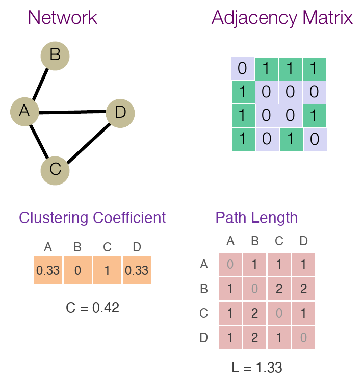
A simple graph and its numerical representation. Four nodes (A–D) are linked by four undirected edges; the corresponding adjacency matrix contains a 1 for each connected pair and 0 otherwise, and is symmetric. From these ingredients we can compute each node’s clustering coefficient (bottom left; network average ) and the shortest path length between every pair of nodes (bottom right; characteristic path length ). (Figure 32.2 from the book. © the authors and MIT Press; reproduced with permission — not covered by this site’s CC-BY license.)
Constructing a brain network means filling in the entries of that matrix. In fMRI the matrix is typically a functional connectome (Chapter 30): correlations between the time series of all node pairs, using Pearson or Spearman correlations, partial correlations, coherence, or mutual information. Because many graph metrics require relatively sparse graphs, the next step is usually to threshold the matrix — removing weak connections — and often to binarize it into an adjacency matrix. Thresholds may be a fixed value, a fixed percentage of retained connections, or a statistical significance level (which raises a multiple comparisons problem across the edge tests, analogous to mass-univariate GLM analysis). The connection density — surviving edges divided by possible edges — measures the resulting sparsity. Thresholding removes weak, potentially spurious connections, sharpens topological structure, and eases computation, but it has real disadvantages: the “right” threshold is rarely obvious, multiplicity grows rapidly with , and — critically — subjects who differ in overall connectivity strength end up with different densities at a fixed threshold, which by itself changes every metric computed downstream. The standard fix is to vary the threshold per subject so that the number of edges (or the density) is held fixed.
Once built, a network can be characterized at several topological scales. Local measures describe individual nodes. A node’s degree counts its neighbors,
kᵢ — degree (number of neighbors) of node i · a_ij — adjacency-matrix entry: 1 if nodes i and j are connected, 0 otherwise
where is the degree of node and the adjacency-matrix entry — 1 if nodes and are connected and 0 otherwise.
Degree is the most common index of centrality — a node’s importance for information transfer — and hence of “hub status” (with strength as the weighted analog). A node’s clustering coefficient asks how many of its neighbors are also neighbors of each other: if nodes , , and are all interconnected they form a closed triangle, and with the number of triangles around node ,
Cᵢ — clustering coefficient of node i · tᵢ — closed triangles containing node i · kᵢ — degree of node i · C — network-average clustering coefficient · N — number of nodes
where is the clustering coefficient of node , the number of closed triangles containing node , its degree, the number of nodes, and the clustering coefficient of the whole network.
The network clustering coefficient is a measure of functional segregation: specialized processing within densely interconnected groups. High clustering implies redundant connections, so losing one node matters less. Betweenness centrality counts the fraction of shortest paths between all node pairs that pass through a node, and the participation coefficient measures how evenly a node’s edges are spread across communities — distinguishing provincial hubs (well connected within their own module) from connector hubs (linking different modules). Global measures summarize the whole network. The shortest path length is the minimum number of edges (or minimum total weight) needed to travel between two nodes, and the characteristic path length
L — characteristic path length of the network · N — number of nodes · Lᵢ — average shortest-path distance from node i to all other nodes
where is the characteristic path length, the number of nodes, and the average shortest-path distance from node to all other nodes.
The characteristic path length indexes functional integration: short paths mean information can be combined rapidly across the network. Related global measures include global efficiency, assortativity (the tendency of high-degree nodes to connect to each other, forming densely interconnected “rich clubs”), and resilience — the ability to keep functioning as nodes and edges are removed. In between sit mesoscale properties: communities (modules) detected by algorithms such as Louvain, Girvan–Newman, or Clauset–Newman–Moore modularity optimization, hierarchical or spectral clustering, and stochastic block models; and, in multilayer networks spanning time points or data types, recruitment and integration of nodes across layers.
These metrics define characteristic types of networks. In a regular network (a lattice or ring) every node has the same degree: clustering is high but so is path length — redundant local communities, inefficient global transmission. In a random (Erdős–Rényi) network every node pair connects with equal probability : both and are low — information travels easily, but the structure is vulnerable and unclustered. A small-world network resembles an ordered network with a few randomly rewired links: high and low , making it simultaneously resilient and efficient. Since Watts and Strogatz’s seminal observation that many social, biological, and technological networks share this property, the brain too has been argued to be small-world — maximizing segregation and integration while minimizing wiring cost. Small-worldness is quantified against a null network:
σ — small-worldness index · C, L — clustering coefficient and characteristic path length of the observed network · C_rand, L_rand — the same metrics averaged over matched random null networks
where and are the clustering coefficient and characteristic path length of the network of interest, and and the same quantities for a matched random null network.
with commonly taken as the cutoff. Other overall structures include core–periphery organization and disassortative networks, in which high-degree nodes preferentially connect to low-degree ones.
Finally, networks can be compared — patients versus controls, or network properties against behavior. So long as the graphs share the same set of nodes, any graph metric can serve as a dependent variable in a GLM regressed on group membership or cognitive performance, or as a feature in machine-learning models (Chapters 37–41). Group differences can be tested nonparametrically with permutation tests that shuffle group labels to build a null distribution for the difference in a metric. And to ask whether a network’s organization is non-random — small-world, core–periphery — the benchmark is a population of simulated random graphs with the same connection density and number of connected nodes, yielding a null distribution for each topological metric of interest.
Hands-on tutorial
In this tutorial you will build a graph from a simulated modular functional connectome, compute the core metrics from the chapter, and see first-hand why threshold choice matters. We simulate 30 nodes organized into three modules (plus a shared global signal that weakly links them), correlate their time series, threshold, and analyze the result.
Step 1 — From connectivity matrix to graph and metrics. We compute the correlation matrix, binarize it at , and compute density, degree, clustering, and characteristic path length.
% Base MATLAB graph objects; CanlabCore on path for the fuller lab
rng(7);                                      % fix the random seed for reproducibility
n = 30; T = 200;                             % n = nodes (regions), T = time points
module  = repelem(1:3, 10)';                 % 3 modules of 10 nodes
g       = randn(1, T);                       % shared global signal
signals = randn(3, T);                       % one latent signal per module
% 0.8 = global-signal weight, 1.2 = noise SD
ts = 0.8 * repmat(g, n, 1) + signals(module, :) + 1.2 * randn(n, T);

R = corr(ts');                               % 30 x 30 functional connectome
A = double(R > 0.3);  A(1:n+1:end) = 0;      % threshold at r > 0.3 + binarize
G = graph(A);

density = numedges(G) / nchoosek(n, 2)       % connection density
deg = degree(G);                             % node degree k_i

t_i = diag(A^3) / 2;  k = sum(A, 2);         % triangles around each node
Ci  = 2 * t_i ./ (k .* (k - 1));  Ci(k < 2) = 0;
C   = mean(Ci)                               % network clustering coefficient

D = distances(G);                            % shortest path lengths d_ij
comp = conncomp(G);  in_cc = comp == mode(comp);
Dcc  = D(in_cc, in_cc);                      % largest connected component
L    = mean(Dcc(Dcc > 0))                    % characteristic path length
import numpy as np, networkx as nx
rng = np.random.default_rng(7) # fix the random seed for reproducibility
n, T = 30, 200 # n = nodes (regions), T = time points
module = np.repeat([0, 1, 2], 10) # 3 modules of 10 nodes
g = rng.standard_normal(T) # shared global signal
signals = rng.standard_normal((3, T)) # one latent signal per module
# 0.8 = global-signal weight, 1.2 = noise SD
ts = 0.8 * g + signals[module] + 1.2 * rng.standard_normal((n, T))
R = np.corrcoef(ts) # 30 x 30 functional connectome
A = (R > 0.3).astype(int) # threshold at r > 0.3 + binarize
np.fill_diagonal(A, 0)
G = nx.from_numpy_array(A)
density = nx.density(G) # connection density
degree = dict(G.degree()) # node degree k_i
C = nx.average_clustering(G) # network clustering coefficient
Gcc = G.subgraph(max(nx.connected_components(G), key=len))
L = nx.average_shortest_path_length(Gcc) # characteristic path length
print(f"density={density:.2f} C={C:.2f} L={L:.2f}")Example output:
density=0.31 C=0.99 L=1.95At , roughly a third of all possible edges survive. Each 10-node module is almost fully interconnected — hence the near-ceiling clustering coefficient — while the sparser between-module links keep the characteristic path length just under 2.
Step 2 — The threshold changes everything. Sweep the threshold and watch density, clustering, and path length co-vary — none of these metrics is interpretable without knowing the density it was computed at.
thr = 0.10:0.05:0.50;                    % thresholds to sweep, lenient -> strict
[dens, Cs, Ls] = deal(zeros(size(thr)));
for i = 1:numel(thr)
    A = double(R > thr(i));  A(1:n+1:end) = 0;
    G = graph(A);
    dens(i) = numedges(G) / nchoosek(n, 2);
    t_i = diag(A^3)/2;  k = sum(A, 2);
    Ci = 2*t_i ./ (k .* (k-1));  Ci(k < 2) = 0;  Cs(i) = mean(Ci);
    D = distances(G);  comp = conncomp(G);
    Dcc = D(comp == mode(comp), comp == mode(comp));
    Ls(i) = mean(Dcc(Dcc > 0));
end
plot(thr, dens, '-o', thr, Cs, '-s', thr, Ls / max(Ls), '-^');
legend({'Density', 'Clustering C', 'Path length L (scaled)'});
xlabel('Correlation threshold');
import matplotlib.pyplot as plt
thresholds = np.arange(0.10, 0.51, 0.05) # thresholds to sweep, lenient -> strict
dens, Cs, Ls = [], [], []
for thr in thresholds:
A = (R > thr).astype(int); np.fill_diagonal(A, 0)
G = nx.from_numpy_array(A)
dens.append(nx.density(G))
Cs.append(nx.average_clustering(G))
Gcc = G.subgraph(max(nx.connected_components(G), key=len))
Ls.append(nx.average_shortest_path_length(Gcc))
plt.plot(thresholds, dens, "-o", label="Density")
plt.plot(thresholds, Cs, "-s", label="Clustering C")
plt.plot(thresholds, np.array(Ls) / max(Ls), "-^", label="Path length L (scaled)")
plt.xlabel("Correlation threshold"); plt.legend()Example output:
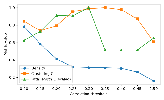
Density and clustering fall as the threshold rises, while the (scaled) characteristic path length climbs as the graph grows sparser and eventually fragments.
Every curve moves together: a “group difference in clustering” at a fixed threshold may be nothing more than a group difference in density. The full labs push further: they plant a connector hub in the network and find it with degree and betweenness centrality, detect communities with greedy modularity optimization and score them against the ground-truth modules, test small-worldness () against density-matched random graphs, and demonstrate that comparing two “subjects” with different overall connectivity strength is confounded at a fixed threshold but fair after density matching.
Open the full Python lab notebook → or download the MATLAB live script, which mirrors it using MATLAB graph objects and CANlab-style workflows.


Thought questions
Node degree, betweenness centrality, and participation coefficient can all be used to call a region a “hub” — yet they can disagree sharply for the same node. Construct (or sketch) a network in which a node has modest degree but very high betweenness, and explain what functional role such a region might play in the brain. Why does the provincial/connector distinction matter for predicting the consequences of a lesion?
A study reports that patients have lower clustering coefficients than controls, using a fixed correlation threshold of applied to every subject. The patients also show globally weaker functional connectivity (e.g., due to greater head motion or vascular differences). Walk through the chain of consequences from weaker correlations to the reported group difference. What analyses would convince you the topological difference is real?
Small-worldness compares a network’s clustering and path length to those of random graphs. What properties should the null networks be matched on (density? degree sequence? connectedness?), and how could a poor choice of null model manufacture — or hide — small-world structure?
Functional connectomes based on correlation are undirected, so all the metrics in this chapter ignore the direction of influence. For which network properties (hubs, communities, efficiency) do you think ignoring directionality is most misleading, and how might metrics computed on a directed effective-connectivity graph (Chapters 35–36) change the picture?
Community-detection algorithms will happily partition any network — including a random one — into “modules.” Drawing on the network-comparison logic of the chapter, design a test for whether the modular structure detected in a resting-state connectome is statistically meaningful rather than an artifact of the algorithm.
Quiz yourself
Q1. In a brain network, what do nodes and edges typically represent, and what distinguishes a connectivity matrix from an adjacency matrix?
Answer: Nodes are brain regions (or voxels) and edges are the functional or structural connections between them. A connectivity matrix holds continuous weighted values representing connection strength; an adjacency matrix is binarized, with 1 for connected and 0 for unconnected node pairs.
Q2. Why are functional connectivity networks undirected, and which methods produce directed brain networks instead?
Answer: Functional connectivity is based on symmetric measures like correlation — the value linking to equals the one linking to — so the matrix is symmetric and the graph undirected. Effective connectivity techniques such as Dynamic Causal Modeling and Granger causality estimate directional influences and yield directed (asymmetric) networks.
Q3. What is connection density, and why is thresholding usually applied before computing graph metrics?
Answer: Density is the number of edges surviving thresholding divided by the maximum possible number of edges — a measure of sparsity. Thresholding removes weak, potentially spurious connections, emphasizes topological structure, and reduces computational burden, and many graph metrics assume relatively sparse graphs.
Q4. Define a node’s degree and clustering coefficient, and say what aspect of brain function each is used to index.
Answer: Degree counts a node’s neighbors and indexes centrality or hub status. The clustering coefficient measures the fraction of a node’s neighbor pairs that are themselves connected (closed triangles); averaged over nodes it indexes functional segregation — specialized processing in densely interconnected groups.
Q5. What is the characteristic path length, and what does a short value imply about a network?
Answer: It is the average shortest path length between all pairs of nodes, . A short characteristic path length implies efficient functional integration — information can be combined rapidly across distributed regions because few edges must be traversed.
Q6. Contrast regular, random, and small-world networks in terms of clustering coefficient and characteristic path length .
Answer: Regular networks (lattices/rings) have high and high — strong local clustering but inefficient global transmission. Random (Erdős–Rényi) networks have low and low . Small-world networks combine the best of both: high with low , quantified by .
Q7. What is the difference between a provincial hub and a connector hub?
Answer: A provincial hub’s connections are mostly local, within its own community or module; a connector hub links nodes in different communities. The participation coefficient — how evenly a node’s edges are distributed across communities — distinguishes them.
Q8. When comparing graph metrics between patient and control groups, why is it problematic if the groups differ in connection density, and what are two remedies?
Answer: Essentially every graph metric depends on density, so a density difference alone can masquerade as a topological difference. Remedies: vary the threshold per subject to fix the number of edges or the connection density (density matching), and use nonparametric permutation tests — shuffling group labels to build a null distribution for the metric difference.
 The book: Elements of Functional Magnetic Resonance Imaging — Wager & Lindquist, MIT Press