Structural Equation and Path Models
Run this code: ⚡ In-browser lab · Colab · MATLAB Online
Overview
Structural equation modeling is a family of techniques for modeling relationships — more formally, the variance–covariance structure — among a set of variables. Where the GLM predicts one outcome from a set of predictors, an SEM specifies a system of equations: multiple predictors, multiple outcomes, and possibly latent factors that are not observed directly but are expressed in the measured variables. The emphasis is on comparing models with different structures and finding one that gives a parsimonious, low-error account of the observed correlations. When all variables are observed (no latent factors), the SEM is called path analysis, and the two most widely used inferences in this framework are tests of mediation — whether the relationship between two variables is transmitted through a third — and moderation — whether one variable changes the strength of the relationship between two others.
Applied to fMRI, SEM is a classic tool for effective connectivity: a set of brain regions is chosen a priori, along with a hypothesized set of directed connections among them. The strength of each connection is a path coefficient — the expected change in activity in one region per unit change in a region that influences it. Writing for the vector of regional activities at one time point, the path model is
y — vector of regional activities at one time point · B — matrix of directed path coefficients (zeros on the diagonal and for absent connections) · ζ — vector of independent errors
where is the vector of regional activities at one time point, the matrix of directed path coefficients (with zeros on the diagonal and wherever no connection is hypothesized), and a vector of independent errors.
Rearranging so appears on only one side, , implies a model covariance matrix
Σ(θ) — model-implied covariance · θ — free parameters (paths and error variances) · B — path matrix · Ψ — error covariance · I — identity matrix
where is the covariance matrix implied by the free parameters (the paths and error variances), the path matrix, the covariance of the errors , and the identity matrix.
Estimation minimizes the discrepancy between this model-implied covariance and the sample covariance, typically by maximum likelihood. Model fit is assessed with a test comparing the two covariance matrices — and, importantly, the logic is reversed from ordinary hypothesis testing: a nonsignificant result means the model is adequate (we cannot reject it), not that it is true or best. Specific edges are tested by comparing nested models with and without the connection using likelihood ratio tests.
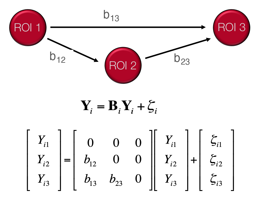
A simple recursive three-variable SEM. ROI 1 influences ROIs 2 and 3, and ROI 2 influences ROI 3; the path coefficients between the three nodes appear as elements of the matrix . (Figure 34.1 from the book. © the authors and MIT Press; reproduced with permission — not covered by this site’s CC-BY license.)
Standard SEM has known limitations for fMRI time series: it assumes observations are independent across time (ignoring temporal autocorrelation, which distorts standard errors), it handles dynamics inflexibly, and it does not incorporate experimental inputs. Extensions such as the unified SEM, which couples a path model with a vector autoregressive model, and the extended unified SEM, which adds experimental inputs, address these gaps. Group analysis is another subtlety: naively concatenating subjects can yield results inconsistent with single-subject analyses, motivating stacked or multilevel SEMs — or simply t-tests across subject-level path estimates, the familiar summary-statistics approach.
Mediation analysis asks whether the effect of an exposure on an outcome is at least partially transmitted through an intervening mediator . The full model is a pair of regressions,
Xᵢ, Mᵢ, Yᵢ — exposure, mediator, outcome for participant i · a — X→M path · b — M→Y path controlling for X · c′ — direct effect of X on Y · i₁, i₂ — intercepts · e — residual errors
where , , and are the exposure, mediator, and outcome for participant ; , , and the path coefficients; and the intercepts; and , the residual errors.
and the reduced model, without the mediator, is , where is its intercept and the total effect. Path is the effect of exposure on mediator, path the effect of mediator on outcome controlling for exposure, and the direct effect — what remains of the relationship once is accounted for. The total effect decomposes exactly:
c — total effect of X on Y · c′ — direct effect (X→Y controlling for M) · ab — indirect effect transmitted through M
where is the total effect of on , the direct effect, and the indirect effect transmitted through the mediator .
so the indirect (mediated) effect is the product , and testing mediation means testing (equivalently, ). The classical Sobel test uses a large-sample normal approximation for the standard error of , but it is overconservative; modern practice uses bootstrap tests — resampling cases, re-estimating thousands of times, and forming confidence intervals and P values from the bootstrap distribution.
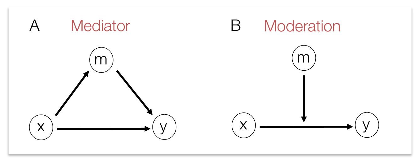
Mediation and moderation. (A) The three-variable path diagram used in mediation analysis: partially explains the relationship between and . (B) Moderation: the value (level) of changes the strength of the – relationship. (Figure 34.2 from the book. © the authors and MIT Press; reproduced with permission — not covered by this site’s CC-BY license.)
Mediation is a natural fit for fMRI because it links experiment, brain, and behavior in one model. A canonical brain-as-mediator design: participants are randomized to a stressful or innocuous challenge (), task-evoked activity in an anterior cingulate cortex (ACC) region is the mediator (), and stressor-evoked heart rate increase is the outcome (). Mediation holds when stress shifts ACC activity (path ) and ACC activity tracks heart rate within groups (path ) strongly enough that the direct effect shrinks relative to . Variables can be organized in other ways too — a brain region mediating the effect of another region on behavior, or one region mediating the link between two other regions. With trial-by-trial data, multilevel mediation estimates paths within person and lets path strengths vary (and be moderated) across people, and mediation effect parametric mapping searches the whole brain for voxels that act as mediators, analogous to a seed analysis.
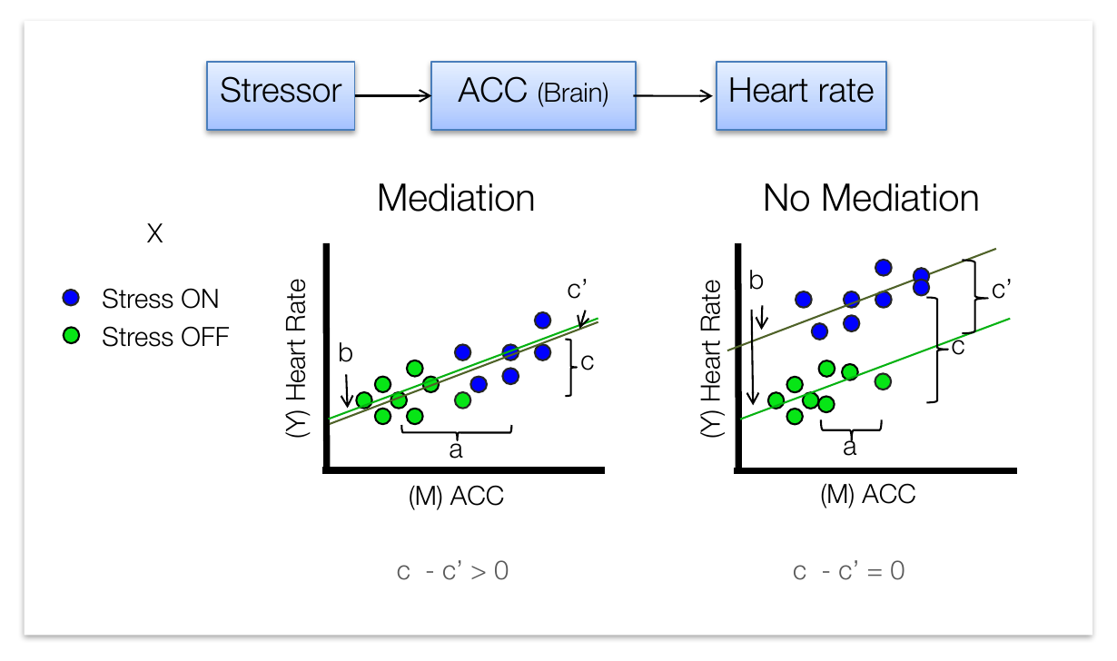
Brain-based mediation. Left: ACC activity mediates the stressor–heart rate relationship — the and effects account for the group difference, so and the parallel fit lines nearly coincide. Right: significant and effects but little mediation, because is small relative to the total effect and a large direct effect remains. (Figure 34.3 from the book. © the authors and MIT Press; reproduced with permission — not covered by this site’s CC-BY license.)
These models are transparent and flexible, but their assumptions deserve respect. The causal reading of requires, among other things, no unmodeled confounding of the mediator–outcome relationship: even when is randomized, is merely observed, so any third variable that drives both and (arousal, attention, global signal) can manufacture a spurious “indirect effect.” These assumptions are easy to state but hard to verify and often violated, which is why mediation in neuroimaging is best framed as pathway discovery and description rather than definitive causal inference — you will create exactly this failure mode in the lab.
Finally, moderation asks a different question: does the – relationship change with the level of a third variable ? It is tested with an interaction term in a standard regression, , where is the intercept, and the main effects of exposure and moderator, and the interaction coefficient — rejecting establishes moderation. The time-series version is the widely used psychophysiological interaction (PPI) analysis: a seed region’s time course, a task variable, and their interaction enter a first-level GLM at every voxel, testing where connectivity with the seed depends on task context. Implementations differ on whether to deconvolve the HRF to form the interaction at the “neural” level (SPM) or interact the convolved signals directly (FSL) — deconvolution is only exact when the HRF is known and the system is linear — and generalized PPI (gPPI) models all task conditions with separate interaction terms for greater power in complex designs.
Hands-on tutorial
In this tutorial you will simulate a brain-as-mediator dataset ( with a direct path), estimate all four paths, and bootstrap the indirect effect — the core mediation workflow. The MATLAB code uses mediation.m from the CANlab Mediation Toolbox; the Python code builds the same analysis from regressions so you can see every moving part.
Step 1 — Simulate mediation data and estimate the paths. We generate observations with true paths , , , then recover them: path from the regression of on , paths and from the regression of on and , and the total effect from the reduced model.
% Requires CanlabCore + MediationToolbox on your MATLAB path
% Adapted from CANlab mediation tutorials (github.com/canlab/MediationToolbox)
rng(42);                               % fix the random seed for reproducibility
n = 200;                               % n = participants (one observation each)
X = randn(n, 1);                       % exposure (e.g., stressor intensity)
M = 0.6 * X + randn(n, 1);             % mediator (e.g., ACC activity), true a = 0.6
Y = 0.2 * X + 0.5 * M + randn(n, 1);   % outcome (e.g., heart rate), b = 0.5, c' = 0.2

% Estimate paths; 'boot' = bootstrap the indirect effect for inference
% (10,000 samples; use at least ~5,000 for stable tails)
[paths, stats] = mediation(X, Y, M, 'boot', 'verbose', 'bootsamples', 10000, ...
    'names', {'Stressor' 'Heart rate' 'ACC'});

% Columns of paths: [a  b  c'  c  a*b]
mediation_path_diagram(stats);         % path diagram with coefficients and stars
import numpy as np
rng = np.random.default_rng(42) # fix the random seed for reproducibility
n = 200 # n = participants (one observation each)
X = rng.standard_normal(n) # exposure (e.g., stressor intensity)
M = 0.6 * X + rng.standard_normal(n) # mediator (e.g., ACC), true a = 0.6
Y = 0.2 * X + 0.5 * M + rng.standard_normal(n) # outcome, true b = 0.5, c' = 0.2
def ols(y, *preds): # OLS betas, intercept first
D = np.column_stack([np.ones(len(y)), *preds])
return np.linalg.lstsq(D, y, rcond=None)[0]
a = ols(M, X)[1] # Path a: M ~ X
cp, b = ols(Y, X, M)[1:3] # Paths c', b: Y ~ X + M
c = ols(Y, X)[1] # Path c: total effect, Y ~ X
print(f"a={a:.3f} b={b:.3f} c'={cp:.3f} c={c:.3f}")
print(f"indirect a*b={a * b:.3f} check c - c'={c - cp:.3f}") # identicalExample output:
a=0.519  b=0.531  c'=0.130  c=0.406
indirect a*b=0.275  check c - c'=0.275
The estimates land near the true values (, , ), and exactly — the decomposition is an algebraic identity for OLS.
Step 2 — Bootstrap inference for the indirect effect. The sampling distribution of is skewed, so we resample cases with replacement, re-estimate each time, and read the 95% confidence interval off the bootstrap distribution. mediation.m does this automatically with the 'boot' option; in Python we write the loop ourselves.
% mediation.m already bootstrapped a*b ('boot', 10,000 samples).
% stats fields hold [a  b  c'  c  a*b] estimates and bootstrap P values:
fprintf('a*b = %3.3f, bootstrap p = %3.4f\n', stats.mean(5), stats.p(5));

% The printed table also reports the Sobel-style parametric test --
% compare: the bootstrap test is typically less conservative.
n_boot = 5000 # bootstrap samples; ~5,000+ for stable CI tails
boot_ab = np.empty(n_boot)
for i in range(n_boot):
idx = rng.integers(0, n, n) # resample cases with replacement
a_i = ols(M[idx], X[idx])[1]
b_i = ols(Y[idx], X[idx], M[idx])[2]
boot_ab[i] = a_i * b_i
lo, hi = np.percentile(boot_ab, [2.5, 97.5])
p_boot = 2 * min((boot_ab <= 0).mean(), (boot_ab >= 0).mean())
print(f"a*b = {a * b:.3f}, 95% bootstrap CI [{lo:.3f}, {hi:.3f}], p = {p_boot:.4f}")Example output:
a*b = 0.275, 95% bootstrap CI [0.176, 0.386], p = 0.0000(None of the 5,000 bootstrap samples crossed zero, so the two-sided P value prints as 0 — report it as .)
The interval should exclude zero decisively — the data were built with real mediation. The full labs push further: they show how an unmodeled confounder of the – relationship produces a significant “indirect effect” when the true path is zero (and how adjusting for the confounder repairs it), and they fit the three-ROI path model of Figure 34.1 by regression equations, testing an individual edge by model comparison.
Open the full Python lab notebook → or download the MATLAB live script, which mirrors it using the CANlab Mediation Toolbox.


Thought questions
In a study where the exposure is randomized but the brain mediator is only measured, which of the paths , , and inherit a causal interpretation from the randomization, and which do not? What kinds of variables could confound the – relationship in a typical fMRI experiment, and what would each do to ?
Two SEMs with reversed arrows (ROI 1 → ROI 2 versus ROI 2 → ROI 1) can imply exactly the same covariance matrix and therefore fit the data equally well. What does this “equivalent models” problem mean for claims of effective connectivity based on SEM fit, and what could you add to the study design to break the symmetry?
Suppose you find significant and paths but the indirect effect is small relative to the total effect , as in the right panel of Figure 34.3. A colleague argues the brain region is “clearly involved” and should be called a mediator anyway. How would you adjudicate, and what additional evidence (statistical or experimental) would strengthen or weaken the mediation claim?
Multilevel mediation estimates paths from trial-by-trial data within each person, while single-level mediation uses one observation per person. What confounds does each approach protect against, and which is vulnerable to individual-difference confounds like age or head motion? When would the two give different answers?
SPM’s PPI deconvolves the seed time course to form the interaction at the “neural” level, while FSL interacts the HRF-convolved signals directly. Lay out the assumptions each approach makes, and explain why the choice matters more for event-related than for blocked designs.
Quiz yourself
Q1. What is the difference between SEM and path analysis?
Answer: Both model relationships among variables with systems of equations, but SEM is the superset: it allows latent (unobserved) factors, correlated errors, and non-recursive relations. Path analysis is the special case in which all variables are observed — as in the three-variable mediation model. Latent variables are seldom used in neuroimaging applications.
Q2. In the mediation model, what do paths , , , and each represent?
Answer: Path is the effect of the exposure on the mediator ; path is the effect of on the outcome controlling for ; path is the direct effect of on that remains after accounting for ; and path is the total effect of on from the reduced model without the mediator.
Q3. Write the decomposition of the total effect, and state what the indirect effect is.
Answer: . The indirect (mediated) effect is the product — the portion of the effect transmitted through — and testing mediation means testing , which is equivalent to testing .
Q4. Why has the bootstrap replaced the Sobel test for inference on ?
Answer: The Sobel test relies on a large-sample normal approximation to the standard error of , but the product of two coefficients has a skewed sampling distribution, making the Sobel test overconservative (P values larger than necessary). Bootstrapping resamples cases, re-estimates many times, and builds confidence intervals and P values from the empirical distribution, respecting the skew.
Q5. In an SEM overall fit test, what does a nonsignificant mean — and what does it not mean?
Answer: The test compares the model-implied covariance matrix with the observed one, so a nonsignificant result means the model’s covariance is not significantly different from the data’s — the model is adequate and cannot be rejected. It does not mean the model is true or the best possible one; other models (including equivalent models with different arrows) may fit as well.
Q6. Give the three ways of organizing variables for a brain mediation analysis described in the chapter.
Answer: (1) A brain region mediates the effect of a task manipulation on an outcome (e.g., dmPFC mediating threat effects on heart rate); (2) a brain region mediates the relationship between another brain region and an outcome (e.g., regions mediating vlPFC’s effect on reappraisal success); (3) a brain region mediates the relationship between two other brain regions, using time-series/trial data (multilevel) or one contrast value per subject (single-level).
Q7. Even with randomized , why can a significant fail to reflect true mediation?
Answer: Because the mediator is observed rather than manipulated, the path (the – relationship controlling for ) can be created by an unmodeled confounder that influences both and . Randomization protects the and paths but not , so the causal “no unmodeled confounding” assumption must hold for the indirect effect to be interpreted causally — which is why mediation in fMRI is often framed as pathway discovery rather than causal proof.
Q8. What is a PPI analysis, and what three regressors define it at the first level?
Answer: Psychophysiological interaction analysis is a time-series moderation test of whether connectivity with a seed region depends on task context. The first-level GLM includes the seed region’s time course (the physiological variable), the task/psychological variable, and their interaction; the interaction term’s parameter map is taken to the group level, and a significant interaction indicates task-modulated connectivity.
 The book: Elements of Functional Magnetic Resonance Imaging — Wager & Lindquist, MIT Press