Dynamic Connectivity
Run this code: ⚡ In-browser lab · Colab · MATLAB Online
Overview
For most of its history, functional connectivity analysis summarized an entire scanning session with a single correlation matrix — static functional connectivity. Over the past decade the field has increasingly asked a different question: does connectivity change over the course of a scan, on time scales of seconds to minutes? In dynamic functional connectivity (DFC) analyses, a central goal is to identify brain states — connectivity patterns that recur across time — among which individuals transition during the scan. States have been observed reliably across groups and individuals, and state-based measures such as the average time spent in each state (dwell time) and the number of transitions between states vary with individual differences such as age and disease status. Findings like these suggest that a single static correlation matrix may be too simplistic to fully capture the interplay between brain regions — though, as we will see, this conclusion has not gone unchallenged.
There are two primary analytic paths, both starting from multivariate time series extracted from atlas regions or ICA components (Chapter 31). In the first, time-resolved connectivity is estimated — for example, a correlation matrix at each time point — and a clustering algorithm groups those matrices into a fixed set of states. In the second, a state-space model such as a hidden Markov model (HMM) estimates the states directly from the time series. Either way, state properties such as dwell time and transition frequency are then extracted and related to stimuli, behavior, or individual differences.
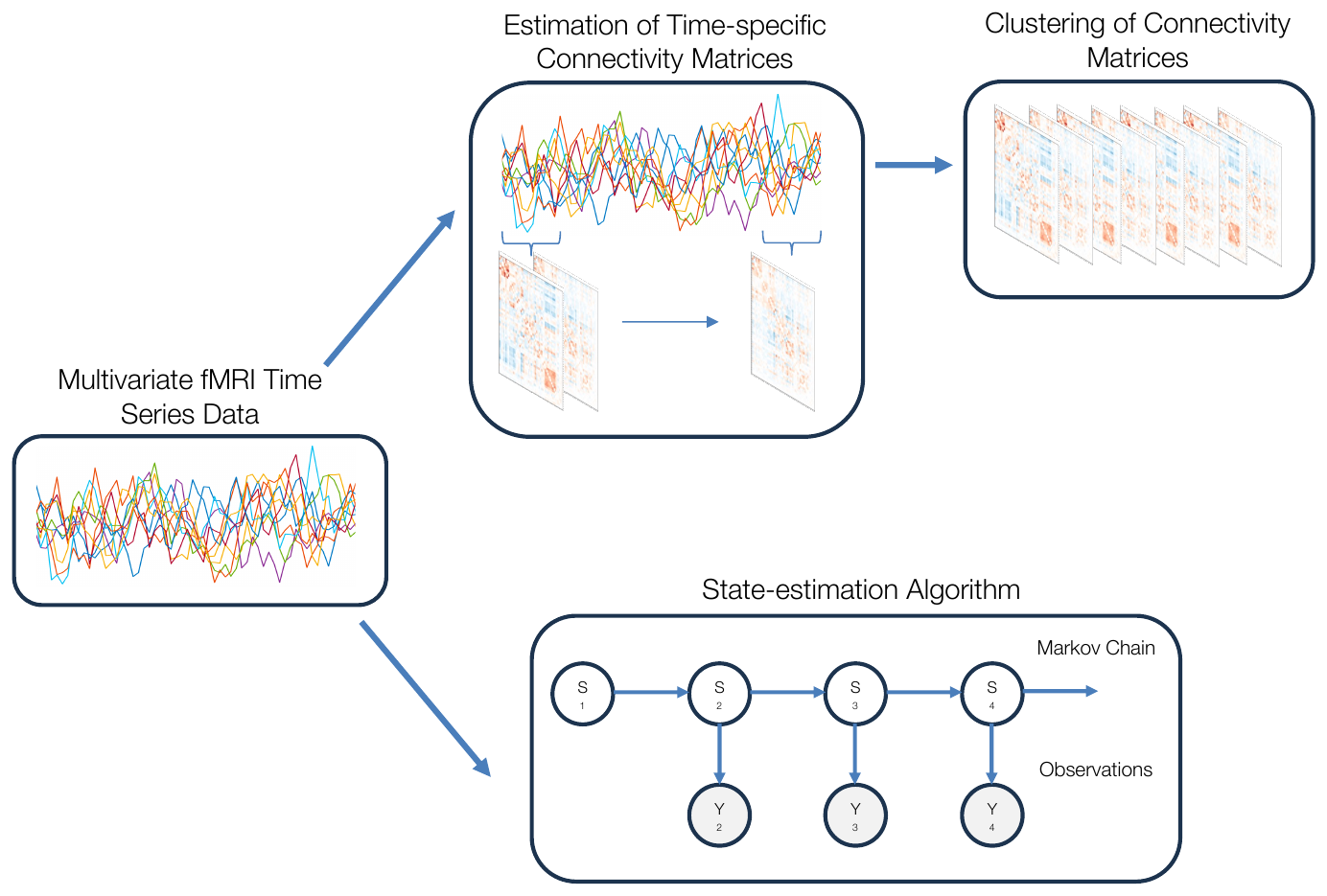
Two common approaches for assessing dynamic functional connectivity. Both begin with multivariate fMRI time series. Top path: time-resolved connectivity matrices (e.g., from sliding windows) are estimated and then clustered into a fixed set of brain states. Bottom path: a state-estimation algorithm such as a hidden Markov model infers the states directly. Properties of the resulting states — dwell time, transition frequency — are then extracted for further analysis. (Figure 33.1 from the book. © the authors and MIT Press; reproduced with permission — not covered by this site’s CC-BY license.)
The workhorse estimator of time-resolved connectivity is the sliding window: compute the connectivity metric over a fixed-length window of the time series (say, 30 TRs), then slide the window one step at a time,
ρ̂ᵢⱼ(t) — windowed correlation between regions i and j, evaluated at time t · xᵢ, xⱼ — the two regions’ time series · t−w+1:t — the w most recent samples · w — window length (in TRs)
where is the estimated correlation between regions and at time , and are the two regions’ time series, denotes the most recent samples, and is the window length in TRs.
The approach is flexible — besides Pearson correlations, common metrics include partial correlations, coherence, mutual information, and multiplication of temporal derivatives — but it has well-known problems. The window length is fixed arbitrarily; all data outside the window are ignored; and windowing smooths over abrupt changes in connectivity. There is a fundamental tradeoff: longer windows give more stable estimates but blur dynamic changes; shorter windows track change but produce noisy, imprecise estimates. A useful rule of thumb is to set the window length to the reciprocal of the lowest frequency (largest wavelength) present in the preprocessed signal.
The tradeoff has an elegant frequency-domain interpretation: applying a moving window is equivalent to convolving the time-resolved connectivity with a fixed window, which acts approximately as a low-pass filter. The Fourier transform of a rectangular window is a sinc function whose main lobe has width — so a sliding-window analysis inherently restricts attention to connectivity fluctuations slower than , and the sinc side-lobes introduce Gibbs ringing (“spectral leakage”) that distorts frequency content and lowers signal-to-noise ratio. Tapered windows reduce spectral leakage, but in simulations built from real resting-state data they were less sensitive to sharp state transitions than rectangular windows — so if abrupt state changes are expected, rectangular windows remain worth considering.
A different strategy is to model the time-varying correlation directly. Dynamic Conditional Correlation (DCC) is an extension of multivariate GARCH models from econometrics, and proceeds in two steps: first, a GARCH model estimates the time-varying variance of each series and produces standardized residuals; second, a dynamic correlation model describes the time-varying correlation matrix of those residuals as a function of past correlations and past errors. A useful intuition for the second step is the exponentially weighted recursion
qᵢⱼ(t) — running (unnormalized) covariance between residual series i and j · zᵢ(t) — standardized GARCH residual of series i at time t · λ — forgetting factor, 0 < λ < 1 · ρ̂ᵢⱼ(t) — time-varying correlation estimate
where is a running (unnormalized) covariance between residual series and , and are the standardized GARCH residuals at time , is the forgetting factor, and is the resulting time-varying correlation estimate.
Recent samples receive weight and older evidence decays geometrically — acts as a “forgetting factor” that plays the same role as the gain in a Kalman filter. Crucially, DCC estimates all of its parameters from the data by maximum likelihood, so no window length (or ) needs to be chosen a priori, and the GARCH step removes time-varying noise variance that would otherwise contaminate the correlations. DCC has been shown to be less susceptible than sliding windows to noise-induced temporal variability, at the price of higher computational cost. Other alternatives include wavelet transform coherence (estimating coherence and phase lag as a function of both time and frequency), coactivation patterns (CAPs; clustering individual fMRI volumes directly), and instantaneous phase synchronization (IPS) based on the Hilbert transform — though IPS requires narrow-band filtering first, which itself acts as an implicit windowing operation.
Once time-resolved connectivity is in hand, the data have expanded enormously — a time series ( time points by regions) becomes a array of time-resolved connections — and the challenge becomes summarizing it. Simple summaries include the mean (essentially the static correlation) and the variance of each connection across time. The more ambitious summary is a set of brain states, most commonly estimated by k-means clustering of the time-resolved matrices. But clustering involves consequential choices. K-means assumes spherical clusters of similar size, is sensitive to outliers, and ignores temporal order entirely — permuting the time points changes nothing. Best practice includes reducing dimensionality (e.g., with PCA) before clustering sparse, high-dimensional data; running multiple centroid initializations; and choosing the number of clusters with an information criterion (AIC/BIC), a permutation or bootstrap null, or Bayesian methods. Methods that respect temporal order — change-point analysis, which partitions the multivariate series at moments of significant covariance change, and HMMs, which model the data with a fixed number of latent states (each a multivariate Gaussian defined by its mean and covariance) plus a transition-probability matrix — will almost certainly do better than order-blind clustering, and both can capture rapid state switches.
Finally, the pitfalls. Time-varying connectivity estimates rest on very few effective degrees of freedom: windows are short, fMRI noise is autocorrelated, and nuisance regression (motion, drift, physiology) removes further degrees of freedom — all of which inflate temporal noise that is easily misread as genuine connectivity change (partial correlations are hit hardest). Fluctuations in arousal and vigilance, and time-varying shifts in the BOLD mean caused by respiration, cardiac activity, transient head motion, or scanner drift, can all produce apparent dynamics. The very existence of resting-state DFC has been controversial: Laumann and colleagues argued that much of the observed “connectivity dynamics” at rest reflects sampling variability, head motion, and drowsiness, so a single static matrix may suffice; and Lindquist showed that sliding-window analysis can reintroduce signals that were previously regressed out — motion-induced signals yielded essentially the same brain states and transitions as the preprocessed data. The lesson is not that dynamics are illusory, but that rigorous statistics — explicit stationary null models, careful denoising, and confound checks — must be part of any dynamic connectivity analysis. The hands-on tutorial below makes exactly this point.
Hands-on tutorial
In this tutorial you will generate convincing-looking “dynamics” from data whose correlation never changes, then test them properly against a stationary null. This is the single most important exercise in dynamic connectivity: learning what pure sampling variability looks like before you interpret anything.
Step 1 — Sliding-window correlation on a static-correlation null. We simulate two time series with a constant true correlation of 0.4 and watch the windowed correlation swing anyway.
% Adapted from Lindquist's Dynamic Correlation Toolbox
% (github.com/canlab/Lindquist_Dynamic_Correlation); see sliding_window.m
rng(33);
T = 600;                                    % number of time points (TRs)
r_true = 0.4;                               % true, constant correlation
w = 30;                                     % sliding-window length (TRs)
Sigma = [1 r_true; r_true 1];              % 2x2 correlation matrix of the generating process
dat = mvnrnd([0 0], Sigma, T);              % correlation NEVER changes

rho = NaN(T, 1);                            % sliding-window correlation
for t = w:T
    c = corr(dat(t-w+1:t, :));
    rho(t) = c(1, 2);
end

figure; plot(rho); yline(r_true, '--');
xlabel('Time (TRs)'); ylabel(sprintf('Windowed correlation (w = %d)', w));
fprintf('Range: [%.2f, %.2f] despite constant true r = %.1f\n', ...
    min(rho), max(rho), r_true);
import numpy as np
import matplotlib.pyplot as plt
rng = np.random.default_rng(33)
T, r_true, w = 600, 0.4, 30 # T = time points (TRs), r_true = true correlation, w = window length
L = np.linalg.cholesky(np.array([[1, r_true], [r_true, 1]])) # 2x2 correlation -> Cholesky factor
dat = rng.standard_normal((T, 2)) @ L.T # correlation NEVER changes
rho = np.full(T, np.nan) # sliding-window correlation
for t in range(w, T + 1):
rho[t - 1] = np.corrcoef(dat[t - w:t].T)[0, 1]
plt.plot(rho); plt.axhline(r_true, ls="--", color="k")
plt.xlabel("Time (TRs)"); plt.ylabel(f"Windowed correlation (w = {w})")
print(f"Range: [{np.nanmin(rho):.2f}, {np.nanmax(rho):.2f}] "
f"despite constant true r = {r_true}")Example output:
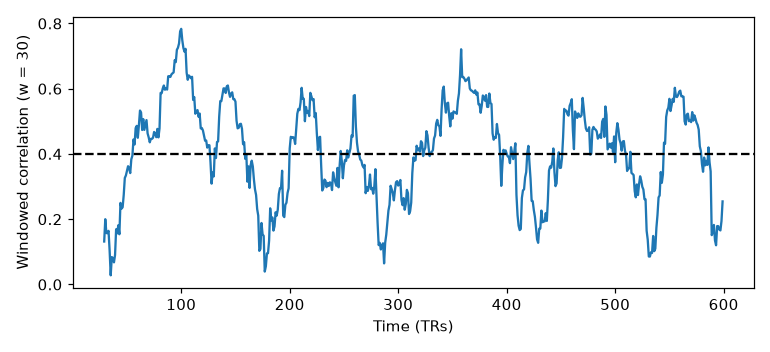
The windowed correlation () swings between about 0 and 0.8 even though the true correlation (dashed line) never moves from 0.4.
Range: [0.03, 0.78] despite constant true r = 0.4The windowed correlation sweeps from near 0 to almost 0.8 — with no true dynamics whatsoever. Cluster matrices like these and you will get “brain states” out of pure noise.
Step 2 — Test against a stationary null. Phase-randomized surrogates keep each series’ power spectrum and their cross-spectrum (hence the static correlation and autocorrelation) but are stationary by construction. We ask: is the observed variability of the windowed correlation larger than a static process would produce?
% Stationary surrogates: same spectra and static correlation, no dynamics
obs = std(rho, 'omitnan');                  % observed test statistic: SD of windowed r
nsur = 200;                                 % number of surrogates; use ~1,000 for publication-grade p-values
nullsd = zeros(nsur, 1);                    % null distribution of the test statistic
F = fft(dat);                               % Fourier coefficients of both series
half = 2:ceil(T/2);                        % positive-frequency bins (excluding DC)
for s = 1:nsur
    ph = zeros(T, 1);
    ph(half) = 2*pi*rand(numel(half), 1);   % same rotation for both series
    ph(T - half + 2) = -ph(half);           % conjugate symmetry
    sur = real(ifft(F .* exp(1i*ph)));
    rs = NaN(T, 1);
    for t = w:T
        c = corr(sur(t-w+1:t, :)); rs(t) = c(1, 2);
    end
    nullsd(s) = std(rs, 'omitnan');
end
p = (1 + sum(nullsd >= obs)) / (nsur + 1);
fprintf('SD of windowed r = %.3f, stationary-null p = %.3f\n', obs, p);
def phase_randomize(dat, rng):
"""Stationary surrogate with the same power- and cross-spectra."""
F = np.fft.rfft(dat, axis=0)
phi = rng.uniform(0, 2*np.pi, size=(F.shape[0], 1)) # same rotation
phi[0] = 0.0 # keep the mean (DC) component real
if dat.shape[0] % 2 == 0:
phi[-1] = 0.0 # keep Nyquist real
return np.fft.irfft(F * np.exp(1j*phi), n=dat.shape[0], axis=0)
def windowed_sd(d):
rs = [np.corrcoef(d[t - w:t].T)[0, 1] for t in range(w, T + 1)]
return np.std(rs)
obs = windowed_sd(dat) # observed test statistic: SD of windowed r
nsur = 200 # number of surrogates; use ~1,000 for publication-grade p-values
null = np.array([windowed_sd(phase_randomize(dat, rng)) for _ in range(nsur)])
p = (1 + np.sum(null >= obs)) / (nsur + 1) # add-one p-value (Phipson & Smyth correction)
print(f"SD of windowed r = {obs:.3f}, stationary-null p = {p:.3f}")Example output:
SD of windowed r = 0.151, stationary-null p = 0.537For this static-null dataset, the test should (correctly) find nothing unusual: the observed variability is entirely typical of a stationary process. The full labs continue the arc: the window-length bias–variance tradeoff, an exponentially weighted (DCC-flavored) estimator racing sliding windows on a true regime-switching signal, and the stationary-null test applied to data with real dynamics — where it correctly rejects.
Open the full Python lab notebook → or download the MATLAB live script, which mirrors it and points to Lindquist’s Dynamic Correlation Toolbox for full DCC estimation.


Thought questions
A colleague analyzes HCP resting-state data (TR = 0.72 s) with a 20-TR sliding window. Using the filter interpretation of windowing, what range of connectivity-fluctuation frequencies can their analysis actually resolve, and how does the rule of thumb — window length equal to the reciprocal of the lowest frequency in the signal — interact with the fact that the data were high-pass filtered at 0.01 Hz during preprocessing?
Laumann and colleagues argued that resting-state “dynamics” largely reflect sampling variability, head motion, and drowsiness. Design an analysis plan that could convince a skeptic that state transitions in your data are neuronal: which null models, physiological measurements, and external validations would you include, and what result pattern would change your own mind in the other direction?
You find that patients dwell longer in a “weakly connected” state than controls do, and the group difference is statistically significant. List at least three non-neuronal explanations for this finding, and describe how you would test or rule out each one.
K-means clustering ignores temporal order — permuting the time points leaves the clusters unchanged — while HMMs and change-point models explicitly use it. Describe a ground-truth scenario where the two approaches would identify very different states, and explain what each method’s assumptions contribute to the disagreement.
Narrow windows, autocorrelated noise, and nuisance regression all reduce the effective degrees of freedom available for each time-resolved connectivity estimate. Explain mechanistically how each one inflates apparent dynamics, and why the problem is worse for partial correlations than for simple correlations.
Quiz yourself
Q1. What is dynamic functional connectivity, and what is a “brain state” in this context?
Answer: Dynamic functional connectivity is time-varying connectivity — changes in the pattern of statistical dependence between regions over the course of a scan, on time scales of seconds to minutes. A brain state is a connectivity pattern that recurs across time (often consistently across subjects); individuals are modeled as transitioning among a fixed set of such states.
Q2. How does the sliding-window technique estimate time-resolved connectivity, and what is the fundamental tradeoff in choosing the window length?
Answer: A connectivity metric (e.g., a correlation matrix) is computed over a fixed-length window of the time series, and the window is moved step-wise across time. Longer windows give more stable estimates but smooth over genuine dynamic changes; shorter windows can detect change but yield noisy, imprecise estimates.
Q3. What is the rule of thumb for choosing a sliding-window length?
Answer: Set the window length to the reciprocal of the frequency of the largest wavelength (i.e., the lowest frequency) present in the preprocessed fMRI signal. This balances estimate reliability against the ability to detect dynamic changes.
Q4. In what sense is a sliding window a low-pass filter, and what do tapered windows fix — and cost?
Answer: A moving window is equivalent to convolving the time-resolved connectivity with the window, whose Fourier transform (a sinc, for a rectangular window) passes only fluctuations slower than roughly 1/window-length. The sinc side-lobes cause Gibbs ringing (spectral leakage). Tapered windows reduce this leakage, but in simulations they were less sensitive to sharp state transitions than rectangular windows.
Q5. Describe the two steps of Dynamic Conditional Correlation (DCC), and two advantages it has over sliding windows.
Answer: Step 1: a GARCH model estimates the time-varying variance of each series and produces standardized residuals. Step 2: a dynamic correlation model expresses the time-varying correlation matrix of those residuals as a function of past correlations and past errors. Advantages: all parameters are estimated from the data (no a priori window length), and removing time-varying variance makes DCC less susceptible to noise-induced variability in correlations. Its main cost is computation.
Q6. What summary measures are typically extracted once brain states are identified, and what are they used for?
Answer: Common measures include the strength of connections within each state, which state is occupied at each moment, the dwell time (average time spent in each state), and the number of transitions between states (change points). These are related to stimuli and task performance within-subject, and to individual differences (e.g., age, disease status) between subjects — which also externally validates the states.
Q7. What assumptions does k-means clustering make about brain states, and why might an HMM be preferable?
Answer: K-means assumes roughly spherical clusters of similar size (it is the maximum-likelihood estimator for a mixture of equal-variance Gaussians), is sensitive to outliers, and completely ignores temporal order. An HMM models each state as a multivariate Gaussian (mean and covariance) plus a transition-probability matrix, so it uses the temporal structure of the data, permits likelihood-based selection of the number of states, and can capture rapid state switching.
Q8. What are the main critiques of resting-state dynamic connectivity findings, and what do they imply for practice?
Answer: Laumann and colleagues argued that much apparent dynamics at rest reflects sampling variability, head motion, and fluctuating sleep state, so a static matrix may suffice. Lindquist showed that sliding windows can reintroduce previously removed signals — motion-induced signals produced essentially the same states and transitions as preprocessed data. Practically: test observed variability against an explicit stationary null, denoise carefully, and evaluate arousal and motion before interpreting states as neuronal.
 The book: Elements of Functional Magnetic Resonance Imaging — Wager & Lindquist, MIT Press