Granger Causal Models
Run this code: ⚡ In-browser lab · Colab · MATLAB Online
Overview
Granger causality mapping uses multivariate time series to infer directed connectivity from temporal precedence: if knowing the past of region improves prediction of the present of region — beyond what ’s own past already provides — we say that Granger causes . The idea originated in economics, where Clive Granger proposed it as a pragmatic, testable stand-in for causality. Unlike structural equation models (Chapter 34) and dynamic causal models (Chapter 35), Granger causality does not require you to specify a structural model of which regions connect to which in advance. It simply asks, for any pair (or set) of regions, whether one series’ history carries predictive information about the other. That makes it more exploratory than confirmatory — potentially most useful in the earlier stages of scientific inquiry, when you do not yet have strong hypotheses about network structure.
The formal machinery is the vector autoregressive (VAR) model. Consider two (possibly multivariate) time series and , assumed stationary. First fit each series on its own past, using models of order , where is the number of lags (past time points) included as predictors:
Xₜ, Yₜ — the two time series at time t · p — model order (number of lags) · Aⱼ, Bⱼ — coefficient matrices for self-influence at lag j · εₜ, ηₜ — zero-mean white-noise innovations
where and are the two (possibly multivariate) time series, is the model order (number of lags), and are coefficient matrices capturing the strength of self-influence at lag , and and are zero-mean white-noise innovations with covariance matrices and .
These models predict each series from its own history alone. Next, stack the two series into and fit a joint model:
Zₜ — the stacked series (Xₜ, Yₜ) · Cⱼ — joint coefficient matrix at lag j · νₜ — white-noise innovation vector · Σ — its covariance, with per-series blocks Σₓₓ, Σᵧᵧ and cross-series blocks Σₓᵧ, Σᵧₓ
where stacks the two series, is the joint coefficient matrix at lag , and is a white-noise innovation vector whose covariance contains the per-series blocks and and the cross-series blocks and .
The joint model lets the current value of each series depend on the past of both. If adding the cross-regressive terms significantly improves the fit — that is, if ’s history predicts after controlling for ’s own history, or vice versa — a Granger-causal relationship is inferred. In practice this is a nested-model comparison: an F-test (or likelihood ratio test) of the full model against the restricted one.
Geweke proposed an elegant way to quantify these influences using the innovation covariances. The total linear dependence between and decomposes into three parts:
F(X,Y) — total linear dependence between X and Y · |·| — matrix determinant · Σ₁, Σ₂ — innovation covariances of the separate models · Σ — innovation covariance of the joint model · F(Y→X), F(X→Y) — directed influences · F(X·Y) — instantaneous dependence
where is the total linear dependence, denotes the matrix determinant, and are the innovation covariances of the separate models, is the innovation covariance of the joint model, and the three terms on the right are defined below.
with the three components defined as
F(Y→X) — influence of Y’s past on X · F(X→Y) — influence of X’s past on Y · F(X·Y) — instantaneous (zero-lag) dependence · Σ₁, Σ₂ — innovation covariances of the separate models · Σₓₓ, Σᵧᵧ — per-series innovation covariances in the joint model · Σ — full joint innovation covariance
where is the directed influence of on , the directed influence of on , and the instantaneous (zero-lag) dependence; and come from the separate models, and , , and from the joint model.
exceeds zero when past values of improve prediction of the current (the joint model’s innovation variance shrinks below the restricted model’s ), and symmetrically for . The third term, , captures instantaneous dependence — shared variance at zero lag that neither history explains. A common summary is the difference , used to infer which region’s history is the more influential.
Applied to fMRI, Granger causality is often used in a whole-brain, seed-based manner. A Granger causality map (GCM) is computed with respect to a single reference region (a seed region or voxel; see Chapter 30): it maps both sources of influence on the seed and targets of influence from the seed across the entire brain — regions that Granger cause the seed, and regions the seed Granger causes.
The approach has been genuinely controversial for fMRI, and the central critique is hemodynamic. BOLD is an indirect, sluggish measure of neuronal activity, and the hemodynamic response function varies across brain regions and individuals (Chapter 18). If region ’s vasculature responds a second faster than region ’s, then ’s BOLD signal will temporally precede ’s even when the underlying neural activity is simultaneous — or even when ’s neural activity leads. Temporal precedence in the signal may reflect hemodynamic, not neuronal, causes, producing spurious directed influence. Proponents have argued that shorter TRs help; critics have argued that Granger causality mapping should not be applied to BOLD data at all. One proposed middle path is to first deconvolve the fMRI time series — removing each region’s estimated hemodynamic response to recover latent neural-like signals — and apply Granger analysis to those. Two further practical cautions: the VAR framework assumes stationarity, so time series spanning distinct states (e.g., baseline and task blocks) should be partitioned into stationary segments or handled with models that account for state transitions; and standard VAR models are linear, though nonlinear extensions exist (e.g., estimating the AR model in a kernel-defined feature space). Finally, remember the scope of the claim: Granger causality indicates only whether activity in one region helps predict activity in another — it makes no statement about how that influence occurs.
Hands-on tutorial
In this tutorial you will build the entire Granger story from scratch on simulated data: first a bivariate VAR(1) system with a genuine directed influence, which Granger tests recover correctly — then a system with perfectly symmetric neural coupling whose two regions have different hemodynamic latencies, which produces a confidently wrong directional inference at the BOLD level.
Step 1 — Simulate a VAR(1) with a true directed influence and test both directions. Region drives region at lag 1 ( receives ), with no influence in the reverse direction.
% Simulate VAR(1): X -> Y at lag 1, no reverse influence
rng(7);                          % seed, for reproducibility
n = 400;                         % time points (think: TRs)
A = [0.5 0.0; ...                % X(t) <- 0.5*X(t-1)
     0.4 0.5];                   % Y(t) <- 0.4*X(t-1) + 0.5*Y(t-1)
Z = zeros(n, 2);                 % columns: X, Y
for t = 2:n
    Z(t, :) = (A * Z(t-1, :)')' + randn(1, 2);   % VAR(1) step + unit-variance noise
end
X = Z(:, 1); Y = Z(:, 2);

% Granger test as a nested-model F-test (lag order p = 1)
% Restricted: Y(t) ~ Y(t-1);  Full: Y(t) ~ Y(t-1) + X(t-1)
T  = (2:n)';                     % usable time points (drop t = 1)
rr = Y(T) - [ones(size(T)) Y(T-1)] * ([ones(size(T)) Y(T-1)] \ Y(T));
rf = Y(T) - [ones(size(T)) Y(T-1) X(T-1)] * ...
            ([ones(size(T)) Y(T-1) X(T-1)] \ Y(T));
F  = ((rr'*rr - rf'*rf) / 1) / ((rf'*rf) / (numel(T) - 3));   % 1 lag tested; 3 params in full model
p  = 1 - fcdf(F, 1, numel(T) - 3);
fprintf('X -> Y:  F = %.1f, p = %.2g\n', F, p);   % large F, tiny p
% Swap X and Y in the code above to test Y -> X (F near 0)
import numpy as np
from statsmodels.tsa.stattools import grangercausalitytests
rng = np.random.default_rng(7) # seed, for reproducibility
n = 400 # time points (think: TRs)
A = np.array([[0.5, 0.0], # X(t) <- 0.5 X(t-1)
[0.4, 0.5]]) # Y(t) <- 0.4 X(t-1) + 0.5 Y(t-1)
Z = np.zeros((n, 2)) # columns: X, Y
for t in range(1, n):
Z[t] = A @ Z[t-1] + rng.standard_normal(2) # VAR(1) step + unit-variance noise
X, Y = Z[:, 0], Z[:, 1]
# grangercausalitytests: does column 2 Granger cause column 1?
res_xy = grangercausalitytests(np.column_stack([Y, X]), maxlag=[1]) # X -> Y
res_yx = grangercausalitytests(np.column_stack([X, Y]), maxlag=[1]) # Y -> X
F_xy, p_xy, *_ = res_xy[1][0]["ssr_ftest"]
F_yx, p_yx, *_ = res_yx[1][0]["ssr_ftest"]
print(f"X -> Y: F = {F_xy:7.1f}, p = {p_xy:.2g} (true influence)")
print(f"Y -> X: F = {F_yx:7.4f}, p = {p_yx:.2g} (no influence)")Example output:
X -> Y:  F =    89.9,  p = 2.3e-19   (true influence)
Y -> X:  F =  0.0001,  p = 0.99   (no influence)
(Exact values differ slightly between the Python and MATLAB versions because their random-number generators differ.)
Step 2 — The HRF confound: equal neural coupling, unequal hemodynamic lags. Now the neural coupling is perfectly symmetric (0.3 in both directions), but region 1’s HRF peaks at ~4 s while region 2’s peaks at ~7 s. (The MATLAB version generates the two response shapes with SPM’s spm_hrf.) At the BOLD level, Granger analysis confidently reports that the fast-HRF region drives the slow-HRF one — a directed influence that does not exist in the neural dynamics.
% Requires SPM12 on the path (for spm_hrf)
TR = 1;                                     % sampling interval (s)
n = 1000;                                   % time points
As = [0.4 0.3; ...                          % symmetric neural coupling:
      0.3 0.4];                             % 0.3 in BOTH directions
Z = zeros(n, 2);
for t = 2:n
    Z(t, :) = (As * Z(t-1, :)')' + randn(1, 2);   % VAR(1) step + unit-variance noise
end

h_fast = spm_hrf(TR, [4 16 1 1 6 0 32]);    % HRF peaking early (~4 s); 1st parameter = delay
h_slow = spm_hrf(TR, [7 16 1 1 6 0 32]);    % HRF peaking late  (~7 s)
sd_noise = 0.05;                            % measurement-noise SD
b1 = conv(Z(:, 1), h_fast); b1 = b1(1:n) + sd_noise * randn(n, 1);
b2 = conv(Z(:, 2), h_slow); b2 = b2(1:n) + sd_noise * randn(n, 1);

% Re-run the nested F-test from Step 1 on the BOLD series, both directions
T = (2:n)';                                 % usable time points
for dir = 1:2
    if dir == 1, tgt = b2; drv = b1; lab = 'fast -> slow';
    else,        tgt = b1; drv = b2; lab = 'slow -> fast'; end
    Xr = [ones(size(T)) tgt(T-1)];          % restricted: own past only
    Xf = [Xr drv(T-1)];                     % full: + other region's past
    rr = tgt(T) - Xr * (Xr \ tgt(T));
    rf = tgt(T) - Xf * (Xf \ tgt(T));
    F  = ((rr'*rr - rf'*rf) / 1) / ((rf'*rf) / (numel(T) - 3));
    fprintf('BOLD %s:  F = %6.1f\n', lab, F);
end
% "fast -> slow" shows a much larger F than "slow -> fast",
% even though the neural coupling is exactly symmetric.
import matplotlib.pyplot as plt
from scipy.stats import gamma
def hrf(t, peak): # double-gamma HRF, peak-normalized
h = gamma.pdf(t, peak) - gamma.pdf(t, 16) / 6
return h / h.max()
t_hrf = np.arange(0, 30, 1.0) # 30-s HRF grid at TR = 1 s
h_fast, h_slow = hrf(t_hrf, 4.0), hrf(t_hrf, 7.0) # peaks ~4 s vs ~7 s
n2 = 1000 # time points (TR = 1 s)
As = np.array([[0.4, 0.3], # symmetric neural coupling:
[0.3, 0.4]]) # 0.3 in BOTH directions
Zn = np.zeros((n2, 2))
for t in range(1, n2):
Zn[t] = As @ Zn[t-1] + rng.standard_normal(2) # VAR(1) step + unit-variance noise
sd_noise = 0.05 # measurement-noise SD
bold1 = np.convolve(Zn[:, 0], h_fast)[:n2] + sd_noise * rng.standard_normal(n2)
bold2 = np.convolve(Zn[:, 1], h_slow)[:n2] + sd_noise * rng.standard_normal(n2)
zs = lambda v: (v - v.mean()) / v.std() # z-score, for plotting on one axis
fig, ax = plt.subplots(figsize=(8, 3))
ax.plot(zs(bold1)[100:200], label="BOLD region 1 (fast HRF)")
ax.plot(zs(bold2)[100:200], label="BOLD region 2 (slow HRF)")
ax.set(xlabel="time (s)", ylabel="z-scored signal",
title="Region 1 leads region 2 — for purely vascular reasons")
ax.legend(frameon=False)
F12, p12, *_ = grangercausalitytests(np.column_stack([bold2, bold1]),
maxlag=[1])[1][0]["ssr_ftest"] # fast -> slow
F21, p21, *_ = grangercausalitytests(np.column_stack([bold1, bold2]),
maxlag=[1])[1][0]["ssr_ftest"] # slow -> fast
print(f"BOLD fast -> slow: F = {F12:6.1f}, p = {p12:.2g}")
print(f"BOLD slow -> fast: F = {F21:6.1f}, p = {p21:.2g}")Example output:
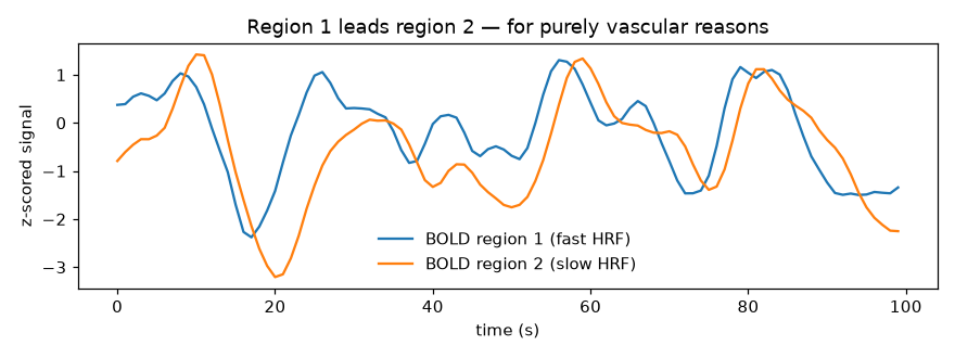
The two observed BOLD series over a 100-s window. Region 1 (fast HRF) visibly leads region 2 (slow HRF) — for purely vascular reasons: the underlying neural coupling is exactly symmetric.
BOLD fast -> slow:  F =  306.4,  p = 5.1e-60
BOLD slow -> fast:  F =   99.4,  p = 2.2e-22
Both directions are “significant” (the symmetric coupling is real), but the fast-HRF region appears to drive the slow-HRF region about three times more strongly than the reverse — an asymmetry that exists only in the measurement, not in the neural dynamics.
The full labs push both steps further: they compute Geweke’s directed-influence measures and from restricted-vs-full residual variances, verify that the neural series in Step 2 are symmetric while the BOLD series are not, and show that deconvolving each region with its own HRF before testing removes the spurious asymmetry (at a real cost in sensitivity).
Open the full Python lab notebook → or download the MATLAB live script, which mirrors it using SPM’s HRF tools.


Thought questions
Granger causality and DCM occupy opposite ends of an exploratory–confirmatory spectrum. Sketch a research program on, say, fear learning in which each method would be used at a different stage, and explain what each contributes that the other cannot.
The core critique of Granger causality for fMRI is that temporal precedence in BOLD may be hemodynamic rather than neuronal. Suppose you observed that region A Granger causes region B during a task but not during rest, with identical scanning parameters. Does the task-vs-rest contrast rescue the causal interpretation? What confounds survive, and what additional data would you want?
Deconvolution promises to remove regional HRF differences before Granger analysis, but it requires estimating each region’s HRF and amplifies noise. Under what combinations of TR, scan duration, and expected neural lag would you judge deconvolution-based Granger analysis worth attempting, and when would you conclude the enterprise is hopeless?
The VAR framework assumes stationarity, yet most task fMRI deliberately alternates between states. Describe two concrete strategies from the chapter for handling a blocked task design, and discuss what each one sacrifices.
“X Granger causes Y” is a statement about prediction, not mechanism. Give an example — from neuroscience or elsewhere — where a variable robustly Granger causes another with no plausible direct influence, and identify the general causal structure (e.g., a common driver with unequal delays) that produces such cases.
Quiz yourself
Q1. In one sentence, what does it mean for time series to Granger cause time series ?
Answer: Past values of improve the prediction of the current value of , over and above what ’s own past values already predict.
Q2. What class of statistical model is used to test for Granger causality, and what key assumption about the time series does it make?
Answer: Vector autoregressive (VAR) models, in which each series is regressed on lagged values of itself and (in the full model) the other series. The framework assumes the series are stationary — constant mean and covariance over time.
Q3. How does Granger causality differ from SEM and DCM in what the analyst must specify in advance?
Answer: SEM and DCM are confirmatory: they require a priori specification of a structural model (which regions are connected), typically comparing a few candidate models. Granger causality requires no structural model — it asks directly whether one region’s history predicts another’s — making it more exploratory.
Q4. In Geweke’s framework, the total linear dependence decomposes into three terms. Name them.
Answer: The directed influence of on (), the directed influence of on (), and the instantaneous influence — dependence at zero lag not explained by either history.
Q5. What is a Granger causality map (GCM)?
Answer: A whole-brain map computed with respect to a single reference (seed) region, showing both regions whose activity Granger causes the seed (sources) and regions the seed Granger causes (targets).
Q6. Why can two regions with identical, simultaneous neural activity still show a significant directed Granger influence in BOLD data?
Answer: Because the hemodynamic response function varies across regions. If one region’s vascular response is faster, its BOLD signal temporally precedes the other’s, and the Granger test attributes this hemodynamic lag difference to directed neural influence — a spurious result.
Q7. What two remedies have been proposed for the hemodynamic confound in fMRI Granger analysis?
Answer: Sampling faster (shorter TRs), which proponents argue mitigates the problem, and deconvolving each region’s estimated HRF from its time series first, so that Granger analysis is applied to reconstructed neural-like signals rather than raw BOLD.
Q8. Your experiment alternates 30-second rest and task blocks. Why is fitting a single VAR across the whole run problematic, and what should you do instead?
Answer: The series is non-stationary — its mean and covariance differ between states — violating the VAR assumption. You should either partition the data into stationary segments (e.g., analyze task and rest separately) or use a model that explicitly accounts for transitions between stationary periods.
 The book: Elements of Functional Magnetic Resonance Imaging — Wager & Lindquist, MIT Press