Chapter 36 Lab — Granger Causal Models (Python) - Elements of fMRI Analysis

In this lab you will build the entire Granger-causality story on simulated data, where the ground truth is known. We follow a five-step arc:

Simulate a VAR(1) system with a genuine directed influence (region X drives region Y)
Test Granger causality in both directions with statsmodels, and see the true direction recovered
Compute Geweke’s directed influence measures from restricted-vs-full model residuals
Create the hemodynamic confound: perfectly symmetric neural coupling, but different HRF latencies in the two regions — and watch Granger analysis confidently report a directed influence that does not exist
Apply a deconvolution remedy, removing each region’s HRF before testing

Because we simulate everything, you can check each inference against the truth — the situation you never enjoy with real BOLD data, and exactly why this confound is so dangerous in practice.

How to run this notebook. Run it in your browser from the tutorial site, in Google Colab, or in a local Jupyter installation. It uses only numpy, scipy, pandas, matplotlib, and statsmodels, and all data are simulated — nothing to download. It accompanies the chapter page.

1. Simulate a VAR(1) system with a true directed influence¶

A first-order vector autoregressive (VAR(1)) model generates each new sample of the bivariate state $Z_t = (X_t, Y_t)^\top$ from the previous sample plus white noise:

Z_t = A\, Z_{t-1} + \epsilon_t, \qquad A = \begin{bmatrix} 0.5 & 0 \\ 0.4 & 0.5 \end{bmatrix}

(1)

Zₜ — bivariate state (Xₜ, Yₜ) at time t · A — 2×2 coupling matrix (row = receiver, column = sender, at lag 1) · εₜ — unit-variance white noise

where $Z_t = (X_t, Y_t)^\top$ is the bivariate state at time $t$ , $A$ is the 2×2 coupling matrix (each row says how one region weights the previous sample of both regions), and $\epsilon_t$ is unit-variance white noise.

Read the coupling matrix row by row: $X_t$ depends only on its own past ( $0.5\,X_{t-1}$ ), while $Y_t$ depends on its own past and on $X$ ’s past ( $0.4\,X_{t-1} + 0.5\,Y_{t-1}$ ). So the ground truth is a one-way influence: X drives Y at lag 1, with no reverse influence. Think of each time step as one TR.

▶ This notebook is interactive. Click the ⏻ power icon at the top right of this page to run it in your browser — no installation needed (the kernel takes ~30–60 s to start the first time). Then run cells top to bottom, starting with the first code cell below: later cells depend on the imports and variables defined earlier, and will error if you skip ahead.

import numpy as np
import pandas as pd
import matplotlib.pyplot as plt
import io, contextlib
from scipy.stats import gamma
from scipy.linalg import toeplitz
from statsmodels.tsa.stattools import grangercausalitytests

rng = np.random.default_rng(7)            # seed, for reproducibility

n = 400                                   # time points (think: TRs)
A = np.array([[0.5, 0.0],                 # X(t) <- 0.5 X(t-1)
              [0.4, 0.5]])                # Y(t) <- 0.4 X(t-1) + 0.5 Y(t-1)

Z = np.zeros((n, 2))                      # columns: X, Y
eps = rng.standard_normal((n, 2))         # unit-variance white noise
for t in range(1, n):
    Z[t] = A @ Z[t - 1] + eps[t]
X, Y = Z[:, 0], Z[:, 1]

fig, ax = plt.subplots(figsize=(9, 3))
ax.plot(X[:120], label="X (driver)", lw=1.2)
ax.plot(Y[:120], label="Y (receiver)", lw=1.2)
ax.set(xlabel="time (samples)", ylabel="signal",
       title="VAR(1) simulation: X drives Y at lag 1")
ax.legend(frameon=False)
plt.tight_layout()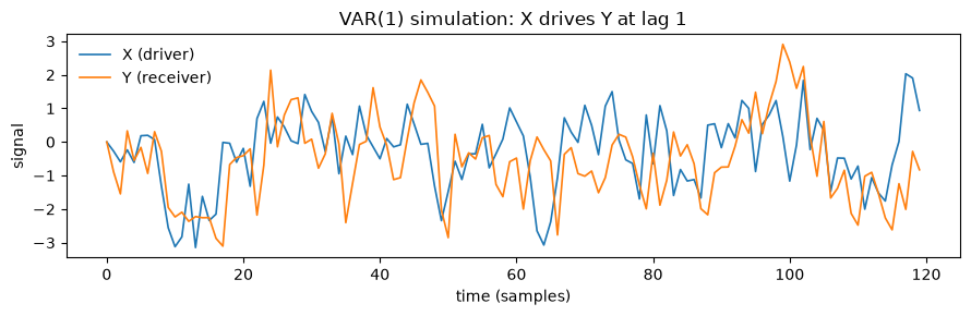

2. Test Granger causality in both directions¶

A Granger test is a nested-model comparison. To ask “does X Granger cause Y?” we compare:

Restricted model: $Y_t \sim Y_{t-1}, \dots, Y_{t-p}$ (Y’s own history only)
Full model: $Y_t \sim Y_{t-1}, \dots, Y_{t-p},\; X_{t-1}, \dots, X_{t-p}$

If the full model fits significantly better (an F-test on the reduction in residual sum of squares), X’s history carries predictive information about Y beyond Y’s own past — X Granger causes Y.

statsmodels.tsa.stattools.grangercausalitytests takes a 2-column array and tests whether the second column Granger causes the first. We wrap it in a small helper that runs one direction quietly and returns the F statistic and P value.

def granger_F(target, driver, lag=1):
    """F test of 'driver Granger-causes target' at the given lag order."""
    data = np.column_stack([target, driver])
    with contextlib.redirect_stdout(io.StringIO()):   # suppress verbose printout
        res = grangercausalitytests(data, maxlag=[lag])
    F, p, _, _ = res[lag][0]["ssr_ftest"]
    return F, p

results = pd.DataFrame(
    [granger_F(Y, X), granger_F(X, Y)],
    index=["X -> Y (true influence)", "Y -> X (no influence)"],
    columns=["F", "p"],
)
print(results.round(4))

                               F       p
X -> Y (true influence)  92.1349  0.0000
Y -> X (no influence)     0.0001  0.9917

The test recovers the truth emphatically: the F statistic for X → Y is enormous (P ≈ 10⁻¹⁹), while Y → X is essentially zero (P ≈ 0.99). Temporal precedence works perfectly here because the “neural” lag (1 sample) is visible at our sampling rate and — crucially — both series are measured the same way, with no differential measurement delay. Hold that thought for Section 4.

3. Geweke’s directed influence measures¶

Geweke quantified directed influence with the ratio of innovation (residual) variances between the restricted and full models. For the influence of $X$ on $Y$ :

F_{X \to Y} = \ln \frac{|\Sigma_2|}{|\Sigma_{yy}|}

(2)

F(X→Y) — directed influence of X on Y · Σ₂ — residual variance of Y predicted from its own past only · Σᵧᵧ — Y’s residual variance in the joint model that also includes X’s past

where $F_{X \to Y}$ is the directed influence of $X$ on $Y$ , $\Sigma_2$ is the residual (innovation) variance of $Y$ predicted from its own past only, and $\Sigma_{yy}$ is $Y$ ’s residual variance in the joint model that also includes $X$ ’s past.

If X’s history helps, the joint model’s residual variance shrinks and $F_{X \to Y} > 0$ ; if it doesn’t help, the ratio is 1 and the measure is 0. In practice, the difference $F_{X \to Y} - F_{Y \to X}$ is often used to infer the net direction of influence — a convention that will matter below.

def geweke(target, driver, lag=1):
    """Geweke directed influence: ln(RSS_restricted / RSS_full)."""
    n = len(target)
    T = np.arange(lag, n)
    ones = np.ones(len(T))
    Xr = np.column_stack([target[T - j] for j in range(1, lag + 1)] + [ones])
    Xf = np.column_stack([target[T - j] for j in range(1, lag + 1)]
                         + [driver[T - j] for j in range(1, lag + 1)] + [ones])
    y = target[T]
    rss_r = np.sum((y - Xr @ np.linalg.lstsq(Xr, y, rcond=None)[0]) ** 2)
    rss_f = np.sum((y - Xf @ np.linalg.lstsq(Xf, y, rcond=None)[0]) ** 2)
    return np.log(rss_r / rss_f)

F_xy, F_yx = geweke(Y, X), geweke(X, Y)
print(f"F_(X->Y) = {F_xy:.4f}")
print(f"F_(Y->X) = {F_yx:.4f}")
print(f"difference (net influence, X->Y positive) = {F_xy - F_yx:.4f}")

F_(X->Y) = 0.2092
F_(Y->X) = 0.0000
difference (net influence, X->Y positive) = 0.2092

4. The hemodynamic confound: equal coupling, unequal HRF lags¶

fMRI does not measure neural activity — it measures BOLD, the neural signal blurred through a sluggish hemodynamic response that varies across brain regions. We now build the critical counterexample from the chapter:

Neural truth: the two regions are coupled perfectly symmetrically — each influences the other with weight 0.3. There is no net directed influence.
Measurement: region 1’s HRF peaks early (~4 s) and region 2’s peaks late (~7 s), a difference well within the range observed across real brain regions.

First, the two HRFs (double-gamma shapes, sampled at TR = 1 s):

def hrf(t, peak, undershoot=16.0, ratio=6.0):
    """Double-gamma HRF, peak-normalized."""
    h = gamma.pdf(t, peak) - gamma.pdf(t, undershoot) / ratio
    return h / h.max()

t_hrf = np.arange(0, 30, 1.0)             # 30-s HRF grid at TR = 1 s
h_fast = hrf(t_hrf, 4.0)                  # region 1: early peak (~4 s)
h_slow = hrf(t_hrf, 7.0)                  # region 2: late peak (~7 s)

fig, ax = plt.subplots(figsize=(7, 3))
ax.plot(t_hrf, h_fast, label="region 1 HRF (peak ~4 s)")
ax.plot(t_hrf, h_slow, label="region 2 HRF (peak ~7 s)")
ax.axhline(0, color="gray", lw=0.5)
ax.set(xlabel="time (s)", ylabel="response (a.u.)",
       title="Two plausible regional HRFs")
ax.legend(frameon=False)
plt.tight_layout()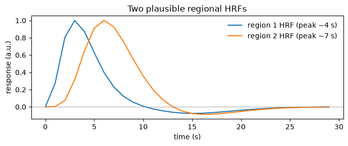

Now simulate the symmetric neural system, then pass each region’s neural series through its own HRF (convolution) and add a little measurement noise to get the “observed” BOLD signals.

rng2 = np.random.default_rng(11)          # separate seed for the confound demo

n2, burn = 1000, 50                       # n2 = time points (TR = 1 s); burn = burn-in samples to discard
A_sym = np.array([[0.4, 0.3],             # region 1 <- itself + region 2, equally
                  [0.3, 0.4]])            # region 2 <- itself + region 1, equally
Zn = np.zeros((n2 + burn, 2))
e2 = rng2.standard_normal((n2 + burn, 2))
for t in range(1, n2 + burn):
    Zn[t] = A_sym @ Zn[t - 1] + e2[t]
Zn = Zn[burn:]                            # discard initial transient
neu1, neu2 = Zn[:, 0], Zn[:, 1]

sd_noise = 0.05                           # measurement-noise SD
bold1 = np.convolve(neu1, h_fast)[:n2] + sd_noise * rng2.standard_normal(n2)
bold2 = np.convolve(neu2, h_slow)[:n2] + sd_noise * rng2.standard_normal(n2)

zs = lambda v: (v - v.mean()) / v.std()
fig, ax = plt.subplots(figsize=(9, 3))
ax.plot(zs(bold1)[100:200], label="BOLD region 1 (fast HRF)", lw=1.2)
ax.plot(zs(bold2)[100:200], label="BOLD region 2 (slow HRF)", lw=1.2)
ax.set(xlabel="time (s)", ylabel="z-scored signal",
       title="Observed BOLD: region 1 leads region 2 — for purely vascular reasons")
ax.legend(frameon=False)
plt.tight_layout()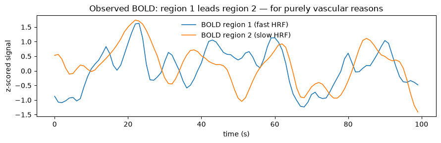

Region 1’s BOLD trace visibly leads region 2’s — not because its neurons fire first, but because its vasculature responds faster. Now run the Granger analysis at both levels: on the (unobservable) neural series, and on the (observable) BOLD series.

rows = {
    "neural: 1 -> 2": (geweke(neu2, neu1), *granger_F(neu2, neu1)),
    "neural: 2 -> 1": (geweke(neu1, neu2), *granger_F(neu1, neu2)),
    "BOLD:   1 -> 2": (geweke(bold2, bold1), *granger_F(bold2, bold1)),
    "BOLD:   2 -> 1": (geweke(bold1, bold2), *granger_F(bold1, bold2)),
}
table = pd.DataFrame(rows, index=["Geweke F", "F stat", "p"]).T
print(table.round(4))

print(f"\nNet influence (Geweke difference, 1->2 minus 2->1):")
print(f"  neural: {geweke(neu2, neu1) - geweke(neu1, neu2):+.4f}   (~0: symmetric, as designed)")
print(f"  BOLD:   {geweke(bold2, bold1) - geweke(bold1, bold2):+.4f}   (strongly positive: SPURIOUS)")

                Geweke F    F stat    p
neural: 1 -> 2    0.1037  108.8252  0.0
neural: 2 -> 1    0.1107  116.6137  0.0
BOLD:   1 -> 2    0.3681  443.2195  0.0
BOLD:   2 -> 1    0.1002  104.9623  0.0

Net influence (Geweke difference, 1->2 minus 2->1):
  neural: -0.0070   (~0: symmetric, as designed)
  BOLD:   +0.2679   (strongly positive: SPURIOUS)

At the neural level the two directed influences are nearly identical (~0.10 each) — the analysis correctly sees a symmetric system. At the BOLD level, the influence of the fast-HRF region on the slow-HRF region is inflated more than threefold relative to the reverse direction, and both directions are “highly significant”. Anyone using the standard net-influence difference would confidently — and wrongly — conclude that region 1 drives region 2. Nothing about the neural dynamics changed; only the measurement did. This is the core of the critique of Granger causality mapping for fMRI: temporal precedence in BOLD can be hemodynamic rather than neuronal.

5. A deconvolution remedy¶

One proposed fix is to deconvolve each region’s HRF from its BOLD series first — reconstructing a neural-like signal — and run the Granger analysis on that. Convolution is a linear operation, $b = H\,z$ , where $H$ is a Toeplitz matrix built from the HRF, so we can invert it with regularized least squares:

\hat{z} = (H^\top H + \lambda I)^{-1} H^\top b

(3)

ẑ — reconstructed neural-like signal · H — Toeplitz convolution matrix built from the HRF · b — observed BOLD series · λ — ridge penalty (damps amplified noise) · I — identity matrix

where $\hat{z}$ is the reconstructed neural-like signal, $H$ the Toeplitz convolution matrix built from the HRF, $b$ the observed BOLD series, $\lambda$ the ridge penalty that damps noise amplification, and $I$ the identity matrix.

The ridge penalty $\lambda$ is needed because deconvolution amplifies high-frequency noise. Here we grant ourselves a luxury real analyses never have: we use each region’s true HRF. In practice the HRF must itself be estimated from the data, adding another layer of uncertainty.

def deconvolve(bold, h, lam=0.05):        # lam = ridge penalty; larger = smoother, more damped
    """Ridge-regularized deconvolution of an HRF from a time series."""
    n = len(bold)
    col = np.zeros(n)
    col[:len(h)] = h
    H = toeplitz(col, np.zeros(n))
    return np.linalg.solve(H.T @ H + lam * np.eye(n), H.T @ bold)

neu1_hat = deconvolve(bold1, h_fast)
neu2_hat = deconvolve(bold2, h_slow)

table2 = pd.DataFrame(
    {"1 -> 2": [geweke(neu2, neu1), geweke(bold2, bold1), geweke(neu2_hat, neu1_hat)],
     "2 -> 1": [geweke(neu1, neu2), geweke(bold1, bold2), geweke(neu1_hat, neu2_hat)]},
    index=["neural (truth)", "BOLD (confounded)", "deconvolved BOLD"],
)
table2["difference"] = table2["1 -> 2"] - table2["2 -> 1"]
print(table2.round(4))

                   1 -> 2  2 -> 1  difference
neural (truth)     0.1037  0.1107     -0.0070
BOLD (confounded)  0.3681  0.1002      0.2679
deconvolved BOLD   0.0145  0.0262     -0.0118

Deconvolution removes the spurious asymmetry: the two directions are again comparable, and the net-influence difference collapses toward zero. But look at the magnitudes — the recovered influences (~0.01–0.03) are far below the neural truth (~0.10). Even with the true HRFs handed to us, regularized deconvolution smooths away much of the lag-1 coupling. The remedy trades a false direction for a large loss of sensitivity — and real analyses must also estimate the regional HRFs, imperfectly. Shorter TRs help on both fronts, which is why sampling rate features so heavily in this debate.

6. Takeaways¶

Granger causality = temporal precedence formalized. X Granger causes Y if X’s past improves prediction of Y beyond Y’s own past, tested as a nested-model F-test within a VAR framework.
It is exploratory. Unlike SEM or DCM, no a priori structural model is needed — useful early in an inquiry, but the output is a statement about prediction, not mechanism.
On true neural-scale signals it works beautifully (Sections 1–3): the correct direction is recovered with overwhelming evidence.
On BOLD it can be confidently wrong (Section 4): regional differences in hemodynamic latency of a second or two — well within the physiological range — masquerade as directed neural influence between symmetrically coupled regions.
Deconvolution and faster sampling are partial remedies (Section 5): they remove the spurious direction but cost sensitivity, and require the regional HRF to be known or estimated.
Stationarity matters: VAR models assume stable means and covariances, so analyze stationary segments (e.g., within task states) or use models that handle state transitions.