Multivariate Brain Analysis: From Maps to Models
Run this code: ⚡ In-browser lab · Colab · MATLAB Online
Overview
For most of this book, analysis has meant brain mapping: fit a separate model at every voxel, with psychological conditions as predictors and that voxel’s activity as the outcome, and aggregate the voxel-wise tests into a statistical map. Maps built this way answer a specific question — is there a non-zero effect of the task in this voxel? — and they answer it stably, because each voxel’s verdict does not depend on what the rest of the brain is doing. But over the past two decades the field has shifted toward a fundamentally different kind of product: integrated, multivariate brain models that specify how to combine measurements across many voxels, regions, or connections to predict the identity or intensity of a mental process. Maps describe the local encoding of information; models attempt to specify the parts of a neural system and how their joint activity predicts mind and behavior.
The mass univariate approach has real strengths — interpretability, the ability to control for other task variables, and a decades-long track record of associating regions with functions. But it also has serious, well-documented weaknesses. It performs one test per voxel, far more tests than independent observations, forcing multiple comparisons correction that decimates power: with typical single-region effect sizes around — where is Cohen’s standardized effect size (mean effect in standard-deviation units) — power can drop as low as 2% in a study of participants. Selecting significant voxels inflates post hoc effect sizes, so published maps are a poor guide to power analyses. Thresholding amplifies instability, so peak coordinates often fail to replicate. And single voxels have low functional specificity: the most pain-selective voxel in the anterior cingulate cortex is also activated by cognitive, motor, language, social, and decision-making tasks — only 12% of the 200+ studies activating it were pain studies. This is why “reverse inference” from a map is so fragile: activation in a region licenses only weak conclusions about which mental process produced it.
Underneath these statistical issues is a deeper mismatch with how the brain encodes information. Mental processes appear to be carried by population codes — patterns of activity across ensembles of neurons, distributed across regions and systems — with only a small proportion of neurons in any one area involved. Testing one voxel at a time is a poor match to that generative process: each voxel’s signal is a noisy, partial reflection of the underlying pattern, so effects in individual voxels are small even when the pattern as a whole is strongly informative. The chapter’s cardiovascular analogy makes the logic intuitive: heart disease is predicted by a profile across many correlated risk factors — genetics, diet, stress, body fat — and that profile can be stable and useful even when no single factor is decisive and even when some factors are only indirectly related to the disease.
Predictive mapping formalizes the alternative. In probability terms, brain mapping estimates — the probability that brain region is active given mental state or symptom . Translation and reverse inference need the opposite: , the probability of the mental state given the brain data. Getting there requires reversing the standard regression equation. Instead of the mass univariate model, fit separately at each voxel ,
yᵥ — voxel v’s time series (time × 1) · X — task design matrix (time × predictors) · βᵥ — voxel v’s regression coefficients · εᵥ — noise at voxel v
where is the measured time series of voxel , the task design matrix (time points × predictors), the voxel-specific regression coefficients, and the noise at that voxel.
a predictive model treats the image as a vector of predictors and the behavior as the outcome:
ŷ — predicted outcome (behavior, state, or condition) · x — brain image as a feature vector (voxels × 1) · w — model weights (one per voxel) · b — intercept (bias)
where is the predicted outcome, the brain image arranged as a vector of features (e.g., voxel activities), the vector of model weights — one per voxel, specifying how voxels jointly contribute to the prediction — and the intercept (bias) term.
Categorical outcomes make this a classification problem (support vector machines, logistic regression, discriminant analysis); continuous outcomes make it a regression problem (ridge, LASSO, elastic net, support vector regression). Some methods — canonical correlation analysis (CCA) and partial least squares (PLS) — extend the idea to multivariate psychological space, mapping patterns of brain features onto patterns of outcomes.
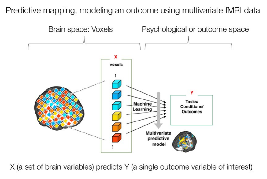
Predictive mapping reverses the standard equation: brain features (voxels) become the predictors , the psychological or clinical variable becomes the outcome , and machine learning estimates the multivariate model that links them. (Figure 37.2 from the book. © the authors and MIT Press; reproduced with permission — not covered by this site’s CC-BY license.)
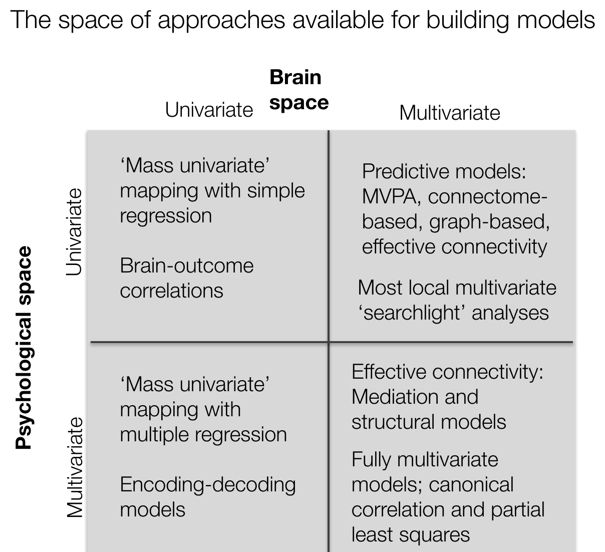
The space of approaches for building models, organized by whether the brain space and the psychological space are univariate or multivariate. Most predictive models are multivariate in brain space and univariate in psychological space; CCA and PLS occupy the fully multivariate cell, and encoding–decoding models sit in the univariate-brain column because the encoding model considers one voxel at a time. (Figure 37.3 from the book. © the authors and MIT Press; reproduced with permission — not covered by this site’s CC-BY license.)
The payoff can be dramatic. Because predictive patterns pool signal over many regions — capturing distributed, outcome-related information while averaging out noise — their effect sizes and reliability far exceed those of single voxels. In the ABCD resting-state data analyzed by Marek, Tervo-Clemmens and colleagues, multivariate prediction yielded effect sizes roughly 4× larger than the top 1% of univariate correlations, cutting required sample sizes by about 16-fold. For task fMRI the gap is even starker: decoding face- vs. shape-viewing in 1,024 Human Connectome Project participants gave a cross-validated effect size of — about 4× the strongest single voxel — with 98% forced-choice accuracy. Predictive models also sidestep voxel-wise multiple comparisons (one model, one test), can show far greater specificity to psychological constructs, and are shareable research products: a weight map makes precise, quantitative predictions that other labs can test on new data, enabling direct replication and generalization tests.
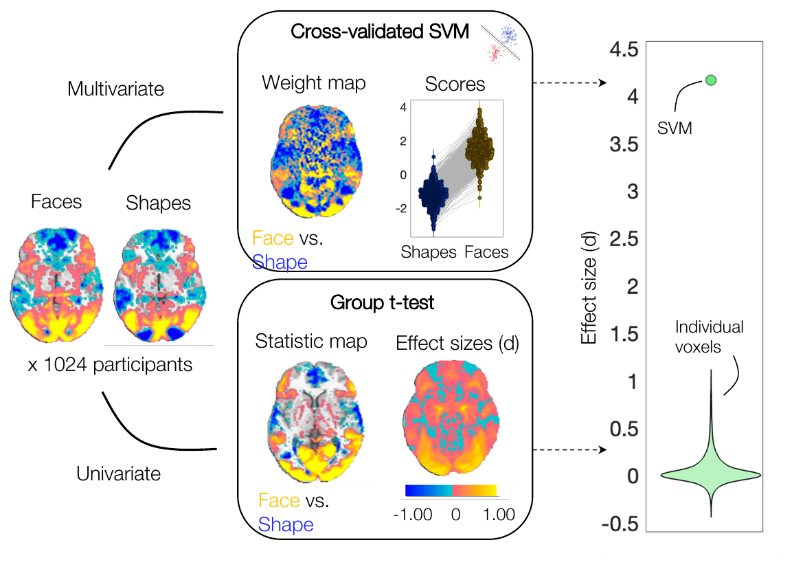
Multivariate models applied to task maps substantially increase effect sizes. Face- vs. shape-viewing images from 1,024 HCP participants analyzed two ways: a voxel-wise group t-test (bottom; voxel effect sizes mostly between and 0.78) and a cross-validated SVM (top), whose pattern scores separate the two conditions with . (Figure 37.5 from the book. © the authors and MIT Press; reproduced with permission — not covered by this site’s CC-BY license.)
A key caution accompanies all this power: the weight map is not an activation map. A linear decoder’s weights describe how to read out the outcome from the data, not where the signal lives. Voxels that carry no task signal at all can receive large weights because they help cancel shared noise (so-called suppressor effects), and genuinely responsive voxels can get near-zero weights if they are redundant with others. To ask the encoding-style question — how does each voxel’s activity covary with the model’s output? — you can transform the weights back into an activation pattern, , where is the data covariance (the Haufe transform). The hands-on tutorial below makes this concrete: you will build a dataset where no single voxel discriminates two conditions, watch a multivariate decoder succeed anyway, and see exactly why its weight map and the encoding map differ.
Finally, turning 100,000+ voxels into a stable, interpretable model is precisely the problem machine learning was built for. Penalization/shrinkage stabilizes estimates when predictors outnumber observations; dimension reduction and feature selection re-represent the data more simply; kernels expand the feature space in controlled ways; and cross-validation assesses predictive accuracy honestly while using data efficiently (Chapters 38–39). Models span a continuum from a single-region regression (interpretable, but limited accuracy) to deep networks with millions of parameters (potentially accurate, but opaque). Whole-brain linear predictive models occupy a productive middle ground — interpretable machine learning that uses information across the brain — and the best models serve double duty: as biomarkers for mental processes and as explanatory accounts of how those processes arise from brain activity.
Hands-on tutorial
In this tutorial you will simulate multivoxel patterns in which the pattern carries information that no single voxel does — a toy population code. The trick is correlated noise: each voxel’s condition difference is buried in fluctuations that are shared across voxels, so a decoder that contrasts voxels against each other can cancel the noise and recover the signal. You will then compare a univariate map with a cross-validated decoder, and see why the decoder’s weights are not a localization map.
Step 1 — Simulate patterns and map them univariately. Two conditions (A and B) differ by a small amount at 60 “signal” voxels; another 60 voxels carry no signal at all. A large global noise source is shared by every voxel, swamping each voxel’s individual effect.
% Simulate: 200 trials x 120 voxels, 2 conditions
% Adapted from CANlab tutorials (github.com/canlab)
rng(7);                                    % seed, for reproducibility
n_tr = 200; V = 120;                       % n_tr = trials, V = voxels
y = repmat([1; -1], n_tr/2, 1);            % condition labels: +1 = A, -1 = B

a = 0.1;                                   % tiny per-voxel signal
sig_vox = 1:60;                            % voxels carrying signal
signal  = zeros(n_tr, V);
signal(:, sig_vox) = repmat(a * y, 1, 60);

g = randn(n_tr, 1);                        % GLOBAL noise, shared by all voxels
g(y == 1)  = g(y == 1)  - mean(g(y == 1)); % condition-independent by design
g(y == -1) = g(y == -1) - mean(g(y == -1));
X = signal + repmat(g, 1, V) ...
    + 0.35 * randn(n_tr, V);               % 0.35 = independent voxel noise SD

% Mass univariate: two-sample t-test at each voxel
[~, p, ~, st] = ttest2(X(y == 1, :), X(y == -1, :));
fprintf('Max |t| = %3.2f; Bonferroni t threshold = %3.2f\n', ...
    max(abs(st.tstat)), tinv(1 - 0.025/V, n_tr - 2));

create_figure('t map'); imagesc(reshape(st.tstat, 10, 12)');
colorbar; title('Univariate t map (no voxel survives correction)');
import numpy as np
import matplotlib.pyplot as plt
from scipy import stats
rng = np.random.default_rng(7) # seed, for reproducibility
n_tr, V = 200, 120 # n_tr = trials, V = voxels
y = np.tile([1, -1], n_tr // 2) # condition labels: +1 = A, -1 = B
a = 0.1 # tiny per-voxel signal
signal = np.zeros((n_tr, V))
signal[:, :60] = a * y[:, None] # voxels 0-59 carry signal
g = rng.standard_normal(n_tr) # GLOBAL noise, shared by all voxels
g[y == 1] -= g[y == 1].mean() # condition-independent by design
g[y == -1] -= g[y == -1].mean()
X = (signal + g[:, None]
+ 0.35 * rng.standard_normal((n_tr, V))) # 0.35 = independent voxel noise SD
# Mass univariate: two-sample t-test at each voxel
t, p = stats.ttest_ind(X[y == 1], X[y == -1])
print(f"max |t| = {np.abs(t).max():.2f}; "
f"Bonferroni t threshold = {stats.t.ppf(1 - 0.025 / V, n_tr - 2):.2f}")
# -> no voxel survives correction
vmax = np.abs(t).max() # symmetric color limits
fig, ax = plt.subplots(figsize=(5.2, 3.4))
im = ax.imshow(t.reshape(10, 12).T, cmap='RdBu_r', vmin=-vmax, vmax=vmax)
ax.set_title('Univariate t map (no voxel survives correction)')
ax.set_xticks([]); ax.set_yticks([])
fig.colorbar(im, ax=ax, label='t value')Example output:
max |t| = 2.26; Bonferroni t threshold = 3.59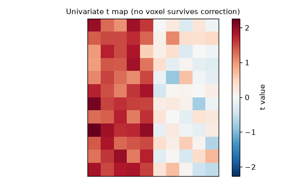
The univariate t map: the signal voxels (left half) trend positive, but no voxel comes close to the Bonferroni-corrected threshold.
Step 2 — Decode the pattern, then compare weights with the encoding map. A cross-validated linear SVM classifies conditions with high accuracy because it weights signal voxels against noise-only voxels, canceling the global noise. The weight map therefore loads on voxels with zero signal — but the Haufe transform recovers the true encoding pattern.
% Cross-validated linear SVM (Statistics and ML Toolbox)
mdl  = fitcsvm(X, y, 'KernelFunction', 'linear');  % linear SVM (box constraint C = 1)
cvm  = crossval(mdl, 'KFold', 5);          % 5-fold cross-validation
fprintf('Decoder accuracy: %3.0f%%\n', 100 * (1 - kfoldLoss(cvm)));

w = mdl.Beta;                              % decoder weights (readout)
A = cov(X) * w;                            % Haufe transform -> encoding map

create_figure('weights vs encoding', 1, 2);
subplot(1,2,1); imagesc(reshape(w, 10, 12)'); colorbar;
title('Decoder weights (suppressors weighted!)');
subplot(1,2,2); imagesc(reshape(A, 10, 12)'); colorbar;
title('Haufe encoding map (signal voxels only)');
from sklearn.model_selection import cross_val_score
from sklearn.svm import LinearSVC
clf = LinearSVC(C=1.0) # C = SVM regularization (1.0 = default)
acc = cross_val_score(clf, X, y, cv=5, n_jobs=1) # cv = 5 folds
print(f"Decoder accuracy: {100 * acc.mean():.0f}%") # >90%
w = clf.fit(X, y).coef_.ravel() # decoder weights (readout)
A = np.cov(X.T) @ w # Haufe transform -> encoding map
import matplotlib.pyplot as plt
fig, axes = plt.subplots(1, 2, figsize=(9, 3)) # side-by-side maps
for ax, m, ttl in zip(axes, [w, A], ["Decoder weights", "Haufe encoding map"]):
im = ax.imshow(m.reshape(10, 12).T, cmap="RdBu_r"); ax.set_title(ttl)
fig.colorbar(im, ax=ax)Example output:
Decoder accuracy: 93%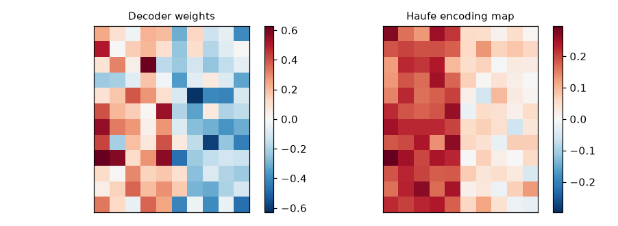
Decoder weights vs. the Haufe-transformed encoding map: the weights load heavily (negatively) on the no-signal voxels, while the encoding map recovers the true signal region (left half).
No voxel discriminates on its own, yet the pattern classifies over 90% of trials correctly — and the noise-only voxels get some of the largest (negative) weights. The full labs walk the whole arc: a two-voxel geometric intuition, the univariate-vs-multivariate accuracy comparison, and side-by-side maps of the true signal, the decoder weights, and the Haufe-transformed encoding pattern.
Open the full Python lab notebook → or download the MATLAB live script, which mirrors it and adds an optional CANlab predict() example on real pain data.


Thought questions
Brain maps estimate while predictive models estimate . For a clinical application — say, an objective marker of chronic pain — explain concretely why the first quantity is insufficient, and what additional properties (sensitivity, specificity, generalization) the second must demonstrate before it is clinically useful.
In the simulation you will run, a decoder assigns large weights to voxels that carry no task signal. Suppose a published study interpreted its decoder weight map as showing “the brain regions that encode pain.” What specific claims would be unwarranted, and how would you re-analyze the data (or redesign the interpretation) to support encoding-style conclusions?
The cardiovascular-risk analogy suggests that predicting an outcome is an easier problem than knowing where to intervene. Where does this distinction bite hardest in neuroimaging — for example, in choosing targets for brain stimulation or neurofeedback — and what kinds of evidence beyond predictive accuracy would you want before intervening on a region because a model weights it heavily?
Multivariate models avoid voxel-wise multiple comparisons because performance is tested with a single number (e.g., cross-validated accuracy). What new risks replace the old ones — think about analytic flexibility in choosing algorithms, features, and cross-validation schemes — and how could a field-wide culture of shared, fixed models (signatures) mitigate them?
Searchlight analysis keeps models local; whole-brain models pool everything; encoding–decoding models fit one voxel at a time and then aggregate predictions. For a study asking whether early visual cortex re-activates percept-specific patterns during imagery, which approach best matches the scientific question, and what would you lose with each of the others?
Quiz yourself
Q1. What is the fundamental difference between a brain map and a brain model?
Answer: A brain map tests, voxel by voxel, whether a psychological variable has a non-zero effect on local activity — it describes the local encoding of information. A brain model specifies how to combine measurements across many brain features to predict the identity or intensity of a mental process or outcome.
Q2. In predictive mapping, what plays the role of predictors and what plays the role of the outcome, and how does this compare with the mass univariate GLM?
Answer: Predictive mapping reverses the mass univariate equation: brain features (e.g., voxel activities) become the predictors, and the behavioral, psychological, or clinical variable becomes the outcome. In the mass univariate GLM it is the opposite — task variables predict each voxel’s activity, one voxel at a time.
Q3. Name three documented weaknesses of mass univariate brain mapping that predictive models help address.
Answer: Any three of: low power after multiple comparisons correction (one test per voxel); inflated post hoc effect sizes due to selection bias; poor reproducibility of thresholded maps and peak coordinates; low test–retest reliability of single-voxel effects; and low functional specificity of individual regions, which undermines reverse inference.
Q4. Which algorithm families are used when the outcome is categorical, and which when it is continuous?
Answer: Categorical outcomes define a classification problem, addressed with classifiers such as support vector machines, logistic regression, discriminant analysis, decision trees, and random forests. Continuous outcomes define a regression problem, addressed with methods such as ridge, LASSO, elastic net, support vector regression, and ordinary multiple regression. Neural networks can handle both.
Q5. How can a multivariate pattern discriminate two conditions when no single voxel does?
Answer: Information can be carried in the joint, relative activity of voxels. When noise is shared (correlated) across voxels, a linear combination that contrasts voxels against each other cancels the common noise while preserving the condition difference — so the pattern’s signal-to-noise ratio can be far higher than any individual voxel’s.
Q6. Why are a linear decoder’s weights not an activation (localization) map, and what is the standard remedy?
Answer: Weights describe an optimal readout, not where signal lives: voxels with no task signal can get large weights because they cancel shared noise (suppressors), and informative voxels can get small weights if redundant. The Haufe transform, , converts the weights into a forward (encoding) pattern showing how each voxel’s activity covaries with the model output.
Q7. In the HCP face vs. shape example, roughly how did the multivariate effect size compare with the best single voxel, and what accuracy did the classifier achieve?
Answer: The cross-validated SVM pattern gave an effect size of about , roughly 4× the strongest individual voxel (max ), and classified face vs. shape image pairs correctly in 98% of participants in a forced-choice test.
Q8. What distinguishes MVPA from predictive modeling, and where do encoding–decoding models fit in the space of approaches?
Answer: MVPA is a family of multivoxel techniques agnostic to purpose — it can be used for prediction or to characterize local similarity structure — whereas predictive modeling specifically identifies and tests the brain basis of an outcome; predictive models can also be built from network edges, graph metrics, or components, not just voxel patterns. Encoding–decoding models fit a separate univariate model per voxel (encoding) and then aggregate voxel-wise predictions into one decoded outcome, so they sit in the univariate-brain column of the approach space.
 The book: Elements of Functional Magnetic Resonance Imaging — Wager & Lindquist, MIT Press