Training and Testing Predictive Models
Run this code: ⚡ In-browser lab · Colab · MATLAB Online
Overview
What makes machine learning distinctive is not the algorithms — it is the question being asked: does the model generalize to new, out-of-sample observations? Generalization depends on simultaneously minimizing two sources of error. Bias is systematic mis-fit: a model too simple to capture the real structure. Variance is imprecision: a model so flexible that it chases noise and gives different answers on every new sample. Feature selection and regularization reduce complexity to keep variance down while keeping bias low. The gold standard for evaluating a model is prospective testing on a brand-new dataset with the model and all its parameters frozen — this yields unbiased estimates of accuracy and probes generalizability across populations, settings, and task designs. But since new datasets are expensive, standard practice is data splitting: learn parameters on training data, evaluate on test data with everything held constant. With no flexibility left at test time, von Neumann’s four-parameter elephant cannot wiggle its trunk.
Valid evaluation requires one crucial condition: the errors in training and test data must be independent. If they are, even wildly overparameterized models can be evaluated fairly; if not, performance estimates are over-optimistic. Independence must be engineered through the design of the split, and there are several classic ways it fails — collectively known as leakage:
Linked observations split across sets — twins, family members, dyads. All members of a group belong on the same side of the split.
Multiple observations per person — trials, events, or images from one participant scattered across training and test. In fMRI this is the cardinal sin: hold out whole subjects (or, for within-person models, whole runs, ideally with a temporal buffer).
Whole-dataset preprocessing before splitting — z-scoring features, regressing out nuisance covariates, or running PCA/ICA on all the data couples the sets together.
Using the outcome before splitting — selecting features by their correlation with on the full dataset is circular analysis, and inflates test performance.
Hidden flexibility in the metric itself — Pearson’s between predicted and observed outcomes re-estimates two parameters (offset and scale) on the test data, hiding systematic over- or under-prediction. It should not be the primary metric reported.
A single split wastes data: less for training means worse models, less for testing means noisier accuracy estimates. Cross-validation resolves the dilemma by resampling: in k-fold cross-validation the data are divided into partitions, each fold serves once as the test set while the model is trained on the rest, and performance is aggregated across all held-out predictions. The final model for future use is then re-trained on the full dataset. Fold count trades off two costs: few folds mean smaller training sets and accuracy biased toward chance; many folds (the extreme is leave-one-out) mean heavily overlapping training sets and high-variance accuracy estimates. Five or ten folds balance these, and stratifying folds on the outcome (and key covariates such as patient vs. control) keeps classes represented and distributions matched. Repeating cross-validation with different random splits and averaging reduces stochastic variability — repeated, stratified 10 × 5-fold cross-validation is a good default for small-to-moderate fMRI studies. Beware class imbalance: with 90 controls and 10 patients, “always say control” is 90% accurate and 100% useless; subsampling, oversampling (e.g., SMOTE), balanced accuracy, and AUC all address this.
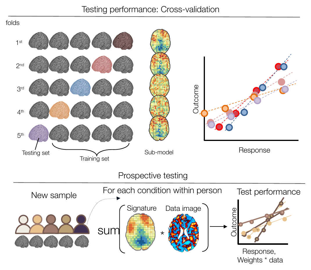
Two stages of model testing. Top: five-fold cross-validation — in each fold a model is trained on 80% of the data and tested on the remaining 20%. Bottom: the trained model is then applied prospectively to new samples, further validating performance and establishing generalizability and boundary conditions. (Figure 39.1 from the book. © the authors and MIT Press; reproduced with permission — not covered by this site’s CC-BY license.)
The rule that makes cross-validation honest is simple to state and easy to violate: every operation applied to the data must happen inside the cross-validation loop. Feature selection, scaling, dimensionality reduction, and — critically — the choice of hyperparameters (an L1/L2 penalty, the number of components) all add flexibility, and if that flexibility touches the test data the accuracy estimate is inflated. Choosing hyperparameters by “run cross-validation for each setting, report the best” is itself overfitting — of the selection procedure rather than the weights. The remedy is nested cross-validation: an inner loop, run within each training set, compares hyperparameter settings and picks a winner; an outer loop evaluates the complete procedure (selection included) on data it has never seen. Even so, final models should ultimately be tested on independent hold-out samples — and then on a widening set of samples differing in population, design, and setting, which maps out the model’s boundary conditions: which characteristics matter for performance and which are ignorable.
How performance is quantified depends on the type of prediction. For classifiers, the confusion matrix tabulates true/false positives and negatives, from which flow sensitivity (TPR, recall), specificity, positive and negative predictive value (PPV is precision), accuracy, and the F1 score . Always inspect per-class accuracy — overall accuracy can be dominated by the majority class — or report balanced accuracy, the mean of per-class accuracies. The ROC curve plots TPR against FPR across decision thresholds, separating discriminability from the threshold choice; the area under the curve (AUC) is the probability that a random positive case outranks a random negative one, equals 0.5 at chance even with imbalanced classes, and is generally preferred to raw accuracy. Discriminability can equivalently be expressed as , the separation between class score distributions in standard deviation units, related to AUC by , where is the standard normal cumulative distribution function.
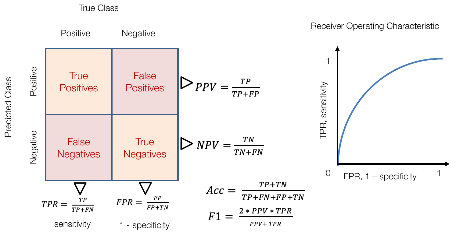
Evaluating classification accuracy. A confusion matrix breaks down true and false positives and negatives, yielding sensitivity (TPR), 1 − specificity (FPR), precision (PPV), NPV, accuracy, and F1. The ROC curve plots TPR against FPR across decision thresholds; the area under it (AUC) measures discriminability independent of threshold. (Figure 39.2 from the book. © the authors and MIT Press; reproduced with permission — not covered by this site’s CC-BY license.)
For regression on continuous outcomes, prefer error-based metrics: mean squared error, RMSE, mean or median absolute error. When predictions come from a model trained without the observation in question, the sum of squared errors is the PRESS, and a particularly interpretable summary is the out-of-sample , which compares the model’s errors to those of simply guessing the training-sample mean :
R²_oos — out-of-sample R² (1 = perfect, 0 = no better than the mean, negative = worse than the mean) · y_i — observed outcome for test observation i · ŷ_i — prediction from a model trained without that observation · ȳ_train — mean outcome in the training sample
where is the observed outcome for test observation , the prediction from a model trained without that observation, and the mean outcome of the training sample.
Unlike in-sample , this can be negative — the model predicts worse than the mean — and it is zero when the model adds nothing. Pearson’s between predicted and observed values, though popular, is biased in complex ways (negatively under cross-validation, optimistically because it re-fits offset and scale to the test data) and should not stand alone.
Finally, many performance measures are, or convert to, effect sizes — , AUC, , Cohen’s — which enable benchmarking across studies (e.g., Pearson’s converts to Cohen’s via ). This matters in fMRI: single-region brain–phenotype associations rarely exceed –0.2, while optimized distributed models reach several-fold larger effects, and within-person task-state prediction can reach very large . Effect sizes computed from continuous model scores (e.g., Cohen’s on SVM distances from the hyperplane) are also more sensitive than thresholded accuracy in small samples. To compare models, apply each to the same independent test observations and compare their errors with the Wilcoxon signed-rank test (two models) or Friedman’s rank sum test (several) — valid even for non-nested models of different complexity, and a practical alternative to AIC/BIC. Inference on cross-validated performance is trickier because training sets overlap across folds; corrections (e.g., Nadeau–Bengio) and permutation tests help, but such inferences should be treated as approximate.
Hands-on tutorial
The full labs run three experiments: the optimism of non-nested hyperparameter selection, subject-level leakage from random splits, and effect-size shrinkage from training to independent test cohorts. Here are the two key moves.
Step 1 — Grouped vs. random cross-validation. We simulate 30 subjects with 8 images each. Each subject has a stable “fingerprint” pattern in the features, but the subject-level label is pure noise — the honest accuracy is 50%. A random split leaks fingerprints across the boundary; a grouped split holds out whole subjects.
% Requires CanlabCore + SPM12; obj is an fmri_data object with one
% subject-level label per image (simulated in the full lab).
% Adapted from CANlab tutorials (github.com/canlab)

% WRONG: random stratified 5-fold CV ignores subject structure --
% images from the same person land in both training and test sets
[cverr, stats] = predict(obj, 'algorithm_name', 'cv_svm', 'nfolds', 5);

% RIGHT: grouped folds -- all of a subject's images share one fold ID
fold_of_subject = repmat(1:5, 1, n_sub / 5);   % subject -> fold (1..5)
wh_folds = fold_of_subject(subject_id)';       % one fold ID per image
[cverr_g, stats_g] = predict(obj, 'algorithm_name', 'cv_svm', ...
    'nfolds', wh_folds);

fprintf('Accuracy -- random split: %.2f | grouped: %.2f\n', ...
    1 - cverr, 1 - cverr_g);                   % inflated vs. ~chance
from sklearn.model_selection import cross_val_score, KFold, GroupKFold
from sklearn.svm import SVC
# X: (240, 100) images; y: subject-level labels; groups: subject ID per image
clf = SVC(kernel="linear") # linear SVM, the fMRI workhorse classifier
acc_rand = cross_val_score(clf, X, y, n_jobs=1,
cv=KFold(5, shuffle=True, random_state=0))
acc_grp = cross_val_score(clf, X, y, groups=groups, n_jobs=1,
cv=GroupKFold(5))
print(f"Accuracy -- random split: {acc_rand.mean():.2f}") # inflated
print(f"Accuracy -- grouped: {acc_grp.mean():.2f}") # ~chance (honest)Example output:
Accuracy -- random split: 0.98
Accuracy -- grouped:      0.48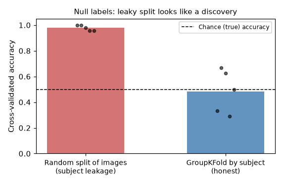
With labels that are pure noise, the random image split reports near-perfect accuracy by memorizing each subject’s fingerprint; grouped folds give the honest answer — chance.
Step 2 — Nested cross-validation for hyperparameters. Choosing a hyperparameter by “run CV for every setting, report the best score” evaluates the winner on the same folds that chose it. Nesting an outer loop around the selection procedure scores the whole pipeline on untouched data.
% Hyperparameter: number of PCR components. Outer loop = evaluation;
% inner loop (grouped CV within training data only) = selection.
ks = [1 2 5 10 20];   % candidate numbers of PCR components (the hyperparameter)
for f = 1:5
    te = (wh_folds == f);  tr = ~te;
    train_obj = get_wh_image(obj, find(tr));
    for i = 1:numel(ks)                        % inner loop: selection
        cverr_inner(i) = predict(train_obj, 'algorithm_name', 'cv_pcr', ...
            'numcomponents', ks(i), 'nfolds', inner_folds, ...
            'error_type', 'mse', 'verbose', 0);
    end
    [~, best] = min(cverr_inner);
    % Refit on all outer-training data with chosen k ('nfolds', 1),
    % then predict the untouched outer test fold
    [~, s] = predict(train_obj, 'algorithm_name', 'cv_pcr', ...
        'numcomponents', ks(best), 'nfolds', 1, 'verbose', 0);
    yfit(te) = obj.dat(:, te)' * s.other_output{1} + s.other_output{2};
end
import numpy as np
from sklearn.model_selection import GridSearchCV, cross_val_score
from sklearn.svm import SVC
rng = np.random.default_rng(6) # seed, for reproducibility
n, p = 40, 50 # n = observations, p = features
X = rng.standard_normal((n, p)) # pure-noise features
y = rng.integers(0, 2, n) # coin-flip labels -> true accuracy is 0.50
grid = {"C": [0.1, 1, 10, 100], # C = SVM regularization strength
"gamma": [1e-3, 1e-2, 1e-1, 1]} # gamma = RBF kernel width; 4 x 4 = 16 settings
inner = GridSearchCV(SVC(kernel="rbf"), grid, cv=3, n_jobs=1) # inner 3-fold selection loop
# NON-NESTED: the same folds pick the hyperparameters AND score the model
score_biased = inner.fit(X, y).best_score_ # optimistic
# NESTED: an outer loop scores the whole selection procedure on new folds
score_nested = cross_val_score(inner, X, y, cv=5, n_jobs=1).mean()
print(f"Non-nested (biased) estimate: {score_biased:.2f}")
print(f"Nested (honest) estimate: {score_nested:.2f}")Example output:
Non-nested (biased) estimate: 0.55
Nested (honest) estimate:     0.50
On null data the non-nested score sits reliably above chance while the nested score hovers at 50% — the gap is pure selection bias. The full labs quantify that gap over repeated simulations, visualize leakage fold by fold, and track how effect sizes shrink from in-sample fits to cross-validation to an independent, distribution-shifted cohort.
Open the full Python lab notebook → or download the MATLAB live script, which mirrors it using CANlab tools.


Thought questions
You are analyzing a twin study of chronic pain with two scans per person. Enumerate every place subject- and family-level dependence could leak into a naive random cross-validation split, and design a splitting scheme that respects all of them. What does your scheme cost you in training-set size and accuracy-estimate precision?
Z-scoring features across the full dataset before splitting introduces leakage even though the outcome variable is never touched. Explain the mechanism, and describe how the same normalization should be implemented inside a cross-validation loop.
Leave-one-out cross-validation uses the most training data and is the least biased toward chance, yet many methodologists recommend 5- or 10-fold instead. Reconstruct the argument in bias–variance terms, and explain when a small dataset plus hyperparameter optimization should push you toward fewer folds.
A colleague reports that their model’s predictions correlate with observed pain in a new cohort and declares it validated. You compute out-of-sample and get -0.4. Explain how both numbers can be true simultaneously, what each metric “forgives,” and what you would report instead.
The chapter recommends testing successful models on a widening set of samples that differ in population, design, and setting to establish boundary conditions. For a brain signature of negative emotion, propose a concrete sequence of increasingly distant test sets, and say what conclusion each generalization success — or failure — would license.
Quiz yourself
Q1. Why can’t a model’s performance be evaluated fairly on the same data used to estimate its parameters?
Answer: Parameter estimation is a form of flexibility that lets the model fit sample-specific noise as well as true signal (overfitting). Performance on the training data is therefore optimistically biased; evaluation requires data whose errors are independent of those used for training.
Q2. In k-fold cross-validation, what happens in each fold, and what is the “final model” once all folds are done?
Answer: The data are split into partitions; in each fold, the model is trained on partitions and evaluated on the held-out one, so every observation is tested exactly once. Performance is aggregated across held-out predictions, and the final model for future use is re-trained on the full dataset.
Q3. Name three distinct sources of leakage that make test performance over-optimistic.
Answer: Any three of: (1) linked observations (twins, dyads, cohorts) split across sets; (2) multiple observations from the same person in both sets; (3) whole-dataset preprocessing before splitting (z-scoring, nuisance regression, PCA/ICA); (4) using the outcome for feature selection before splitting (circular analysis); (5) metrics like Pearson’s that fit new parameters (offset, scale) on the test data.
Q4. What is the tradeoff in choosing the number of cross-validation folds?
Answer: Fewer folds mean smaller training sets, so models underperform and accuracy is biased toward chance. More folds (up to leave-one-out) reduce that bias but make training sets overlap heavily, inflating the variance of the accuracy estimate. Five- or ten-fold cross-validation balances the two, and repeated stratified CV (e.g., 10 × 5-fold) reduces split-to-split variability.
Q5. What problem does nested cross-validation solve, and what do the inner and outer loops do?
Answer: It prevents hyperparameter selection from inflating accuracy estimates. The inner loop, run entirely within each training set, compares modeling choices (e.g., penalty strength, number of components) and selects a winner; the outer loop evaluates the complete procedure — selection included — on held-out data. Selection and evaluation thus rely on independent observations.
Q6. With 90% of observations in one class, why is overall accuracy misleading, and which two metrics handle imbalance better?
Answer: A classifier that always predicts the majority class achieves 90% accuracy while being 0% accurate on the minority class. Balanced accuracy (the average of per-class accuracies) and AUC (which equals 0.5 at chance regardless of base rates) are not fooled by imbalance.
Q7. Why is Pearson’s between predicted and observed outcomes a poor primary metric, and what should be reported instead?
Answer: Computing on the test data implicitly fits two new parameters — an offset and a scale — so a model that systematically over- or under-predicts is not penalized; is also negatively biased under cross-validation. Report error-based metrics (RMSE, MAE) and out-of-sample , which can go negative when the model predicts worse than the training mean.
Q8. How can a classifier’s performance be expressed as a continuous effect size, and why would you want to?
Answer: Compute each observation’s continuous model score (e.g., distance from the SVM hyperplane) and calculate Cohen’s between classes, or use /AUC, which are directly related (). Continuous effect sizes avoid the information loss of binary thresholding, are more stable in small samples, and allow benchmarking against familiar standards across models and studies.
 The book: Elements of Functional Magnetic Resonance Imaging — Wager & Lindquist, MIT Press