This lab makes the core principles of machine learning concrete with small simulations: the U-shaped test error curve and the bias–variance tradeoff, ridge vs. lasso regularization paths, cross-validation done wrong vs. right (feature-selection leakage), and ROC curves for evaluating classifiers.
How to run this notebook. You can run it directly in your browser (each cell takes a few seconds), open it in Colab with the badge on the chapter page, or download and run it locally. Everything uses numpy, scikit-learn, and matplotlib on simulated data — no fMRI files needed. If anything is unfamiliar, revisit the chapter page first.
▶ This notebook is interactive. Click the ⏻ power icon at the top right of this page to run it in your browser — no installation needed (the kernel takes ~30–60 s to start the first time). Then run cells top to bottom, starting with the first code cell below: later cells depend on the imports and variables defined earlier, and will error if you skip ahead.
import numpy as np
import matplotlib.pyplot as plt

rng = np.random.default_rng(2026)             # seed for reproducibility
plt.rcParams["figure.dpi"] = 100              # crisper inline figures
1. Overfitting and the U-shaped test error curve
Machine learning judges models by how well they predict new data. To see why that matters, we simulate observations from a smooth true function, , and fit polynomials of increasing degree — a simple dial for model complexity. We fit on a small training set and evaluate on an independent test set.
Training error can only go down as complexity grows: a more flexible model always fits the points it was trained on more closely.
Test error is U-shaped: it falls while flexibility captures real structure (reducing bias), then rises as the model starts fitting noise (increasing variance).
f_true = lambda x: np.sin(2 * x)              # true function generating the data
sigma = 0.4                                   # noise SD

n_train, n_test = 30, 400                     # small training set, large test set
x_train = 4 * rng.random(n_train)
y_train = f_true(x_train) + sigma * rng.standard_normal(n_train)
x_test = 4 * rng.random(n_test)
y_test = f_true(x_test) + sigma * rng.standard_normal(n_test)

degrees = np.arange(1, 13)                    # complexity levels to sweep
train_mse, test_mse, fits = [], [], {}
for d in degrees:
    p = np.polyfit(x_train, y_train, d)        # fit uses training data ONLY
    train_mse.append(np.mean((y_train - np.polyval(p, x_train)) ** 2))
    test_mse.append(np.mean((y_test - np.polyval(p, x_test)) ** 2))
    fits[d] = p

fig, axes = plt.subplots(1, 2, figsize=(11, 4))
xx = np.linspace(0, 4, 300)
axes[0].plot(x_train, y_train, "ko", ms=4, label="training data")
axes[0].plot(xx, f_true(xx), "g-", lw=2, label="true function")
for d, style in [(1, "b--"), (3, "r-"), (12, "m:")]:
    axes[0].plot(xx, np.polyval(fits[d], xx), style, label=f"degree {d}")
axes[0].set(ylim=(-2, 2), xlabel="x", ylabel="y", title="Fits of increasing complexity")
axes[0].legend(fontsize=8)

axes[1].plot(degrees, train_mse, "b.-", label="Training error")
axes[1].plot(degrees, test_mse, "r.-", label="Test error")
axes[1].axhline(sigma**2, color="gray", ls=":", label="Irreducible noise ($\sigma^2$)")
axes[1].set(xlabel="Polynomial degree (complexity)", ylabel="MSE",
            title="Test error is U-shaped")
axes[1].legend(fontsize=8)
plt.tight_layout()

best = degrees[int(np.argmin(test_mse))]
print(f"Best test-set degree: {best}  (true function is smooth and sine-like)")
Best test-set degree: 7 (true function is smooth and sine-like)
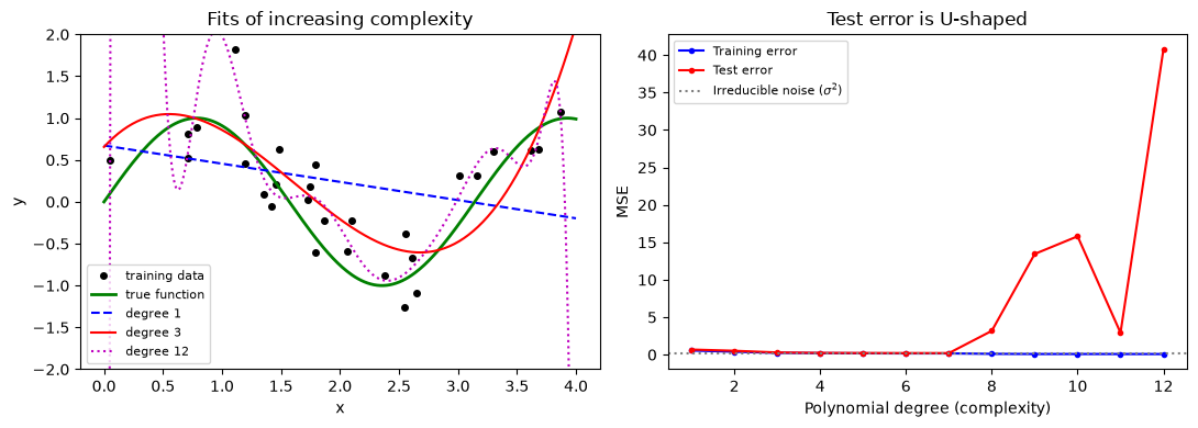
The degree-1 fit underfits (high bias: systematically wrong everywhere), while the degree-12 fit overfits (high variance: it chases individual noisy points). The best test error lands at moderate complexity — and no model beats the irreducible noise floor .
2. The bias–variance tradeoff, visualized
Bias and variance are statements about what happens across repeated samples. We redraw the training set many times, refit each model, and overlay the fitted curves. A simple model gives nearly the same (wrong) curve every time — high bias, low variance. A complex model gives wildly different curves each time — low bias, high variance.
n_sims = 50                                   # number of re-drawn training sets
xx = np.linspace(0.1, 3.9, 200)               # grid for evaluating fitted curves
show_degrees = [1, 3, 12]                     # underfit, about right, overfit

fig, axes = plt.subplots(1, 3, figsize=(12, 3.6), sharey=True)
for ax, d in zip(axes, show_degrees):
    curves = np.empty((n_sims, xx.size))
    for s in range(n_sims):
        xs = 4 * rng.random(n_train)
        ys = f_true(xs) + sigma * rng.standard_normal(n_train)
        curves[s] = np.polyval(np.polyfit(xs, ys, d), xx)
    ax.plot(xx, curves.T, color="steelblue", alpha=0.15, lw=1)
    ax.plot(xx, f_true(xx), "g-", lw=2)
    ax.plot(xx, curves.mean(0), "r--", lw=2)
    bias2 = np.mean((curves.mean(0) - f_true(xx)) ** 2)
    var = curves.var(0).mean()
    ax.set(ylim=(-2, 2), xlabel="x",
           title=f"degree {d}\nbias$^2$={bias2:.3f}, var={var:.3f}")
axes[0].set_ylabel("y")
fig.suptitle("Blue: 50 refits on new samples.  Green: truth.  Red dashed: average fit.", y=1.04)
plt.tight_layout()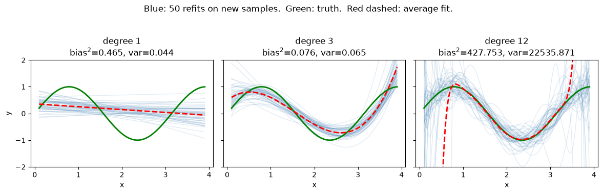
The printed decomposition mirrors the picture: degree 1 has large bias² and tiny variance; degree 12 has near-zero bias² and large variance; degree 3 balances the two. Expected test error ≈ bias² + variance + , which is exactly why the test error curve in Section 1 is U-shaped.
3. Regularization: ridge and lasso coefficient paths
When features are many and correlated — the norm in fMRI — regularization controls complexity continuously instead of by discrete model choice. We minimize a penalized loss with
L2 / ridge: — shrinks all coefficients smoothly toward zero,
L1 / lasso: — drives the least useful coefficients exactly to zero (sparsity).
We simulate 40 correlated features of which only 5 truly matter, then trace every coefficient as the regularization strength (called alpha in scikit-learn) varies.
from sklearn.linear_model import Ridge, lasso_path

n, p, p_true = 80, 40, 5                      # n = observations, p = features, p_true = truly predictive
# correlated design: features share a common latent factor
latent = rng.standard_normal((n, 1))
X = 0.6 * latent + rng.standard_normal((n, p))
X = (X - X.mean(0)) / X.std(0)
w_true = np.zeros(p); w_true[:p_true] = [3, -2.5, 2, -1.5, 1]   # only the first 5 features matter
y = X @ w_true + rng.standard_normal(n)

alphas = np.logspace(-2, 3, 60)               # regularization strengths (lambda), log-spaced

# Ridge path: refit at each alpha
ridge_coefs = np.array([Ridge(alpha=a).fit(X, y).coef_ for a in alphas])

# Lasso path (efficient built-in path algorithm)
alphas_lasso, lasso_coefs, _ = lasso_path(X, y, alphas=alphas / n)

fig, axes = plt.subplots(1, 2, figsize=(11, 4), sharey=True)
for j in range(p):
    c = "crimson" if w_true[j] != 0 else "lightgray"
    axes[0].plot(np.log10(alphas), ridge_coefs[:, j], color=c, lw=1.2)
    axes[1].plot(np.log10(alphas_lasso * n), lasso_coefs[j], color=c, lw=1.2)
axes[0].set(title="Ridge (L2): smooth shrinkage, nothing exactly 0",
            xlabel="log10($\lambda$)", ylabel="coefficient")
axes[1].set(title="Lasso (L1): sparse — coefficients hit exactly 0",
            xlabel="log10($\lambda$)")
for ax in axes: ax.axhline(0, color="k", lw=0.5)
plt.tight_layout()

n_nonzero = (np.abs(lasso_coefs) > 1e-8).sum(0)
print("Lasso nonzero coefficients along the path (high to low lambda):")
print(np.array(sorted(set(n_nonzero))))
Lasso nonzero coefficients along the path (high to low lambda):
[ 0 1 3 5 6 7 10 11 13 19 23 25 28 30 31 32 33 36 37 38 39 40]
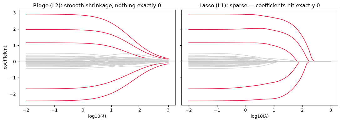
Red paths are the 5 truly predictive features; gray paths are pure noise. Ridge shrinks everything smoothly but keeps all 40 features; lasso zeroes out the noise features over a wide range of , recovering a sparse model. With strongly correlated features, though, lasso picks one arbitrary representative per correlated set — in whole-brain models this produces scattered “speckles,” motivating elastic net, structured penalties (GraphNet), and LASSO-PCR on component scores.
In practice is a hyperparameter chosen by cross-validation — which brings us to the most important cautionary tale in this lab.
4. Cross-validation done WRONG vs. right
Cross-validation is only valid if every data-dependent choice — feature selection, scaling parameters, hyperparameter tuning — is made using training folds only. A classic mistake is to select the features most correlated with the outcome using the whole dataset, and only then cross-validate. The selection step has already peeked at the test folds.
To show how bad this is, we use features that are pure noise: true generalization accuracy is exactly 50%. Any excess is optimism created by leakage.
from sklearn.model_selection import StratifiedKFold

n, p, k_feats = 50, 2000, 20                  # n = participants, p = noise features, k_feats = features kept

def top_k_features(Xa, ya, k):
    """Indices of the k features most correlated (|r|) with the outcome."""
    Xc = Xa - Xa.mean(0)
    r = (Xc.T @ (ya - ya.mean())) / (np.sqrt((Xc**2).sum(0)) *
                                     np.sqrt(((ya - ya.mean())**2).sum()) + 1e-12)
    return np.argsort(np.abs(r))[-k:]

def fit_predict(Xtr, ytr, Xte):
    """Least-squares linear classifier: sign(X w)."""
    w = np.linalg.lstsq(Xtr, ytr, rcond=None)[0]
    return np.sign(Xte @ w)

def cv_accuracy(X, y, select_first, seed=0):
    sel_all = top_k_features(X, y, k_feats) if select_first else None
    skf = StratifiedKFold(10, shuffle=True, random_state=seed)
    correct = 0
    for tr, te in skf.split(X, y):
        sel = sel_all if select_first else top_k_features(X[tr], y[tr], k_feats)
        correct += np.sum(fit_predict(X[tr][:, sel], y[tr], X[te][:, sel]) == y[te])
    return correct / len(y)

n_datasets = 20                               # simulated datasets; more repeats -> smoother histograms
acc_wrong, acc_right = [], []
for s in range(n_datasets):
    Xs = rng.standard_normal((n, p))            # PURE NOISE features
    ys = np.repeat([1.0, -1.0], n // 2)
    acc_wrong.append(cv_accuracy(Xs, ys, select_first=True, seed=s))
    acc_right.append(cv_accuracy(Xs, ys, select_first=False, seed=s))
acc_wrong, acc_right = np.array(acc_wrong), np.array(acc_right)

print(f"WRONG (select on all data, then CV): {acc_wrong.mean():.1%} "
      f"(range {acc_wrong.min():.0%}-{acc_wrong.max():.0%})")
print(f"RIGHT (select inside each fold):     {acc_right.mean():.1%} "
      f"(range {acc_right.min():.0%}-{acc_right.max():.0%})")
print(f"True accuracy of any model here:     50.0% (features are pure noise)")
print(f"Average optimism from leakage:       {(acc_wrong - acc_right).mean():+.1%}")

plt.figure(figsize=(6, 3.5))
plt.hist(acc_wrong, bins=np.arange(0.3, 1.01, 0.04), alpha=0.7,
         label="WRONG: selection before CV", color="crimson")
plt.hist(acc_right, bins=np.arange(0.3, 1.01, 0.04), alpha=0.7,
         label="RIGHT: selection inside CV", color="steelblue")
plt.axvline(0.5, color="k", ls=":", label="chance")
plt.xlabel("10-fold CV accuracy"); plt.ylabel("count of simulated datasets")
plt.title("Feature-selection leakage on pure-noise data")
plt.legend(fontsize=8); plt.tight_layout()
WRONG (select on all data, then CV): 91.2% (range 80%-100%)
RIGHT (select inside each fold): 54.1% (range 38%-74%)
True accuracy of any model here: 50.0% (features are pure noise)
Average optimism from leakage: +37.1%
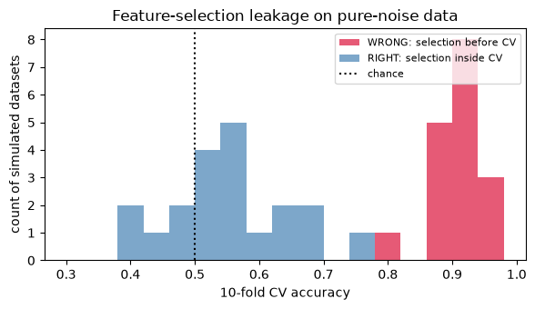
On data with no signal whatsoever, the leaky pipeline reports accuracies far above chance — often 75–90% — while the correct pipeline hovers around 50%. The gap is the optimism bought by letting the test folds influence feature selection. With real data the same bias operates silently on top of any true signal, inflating published accuracies. The rule: cross-validation must wrap the entire pipeline, including selection, scaling, and hyperparameter tuning (nested CV; Chapter 39).
5. ROC curves and AUC
Accuracy at a single threshold hides how a classifier trades off sensitivity against specificity. The ROC curve sweeps the decision threshold across all values of a continuous score, plotting the true positive rate against the false positive rate. The area under the curve (AUC) summarizes separability: 0.5 = uninformative, 1.0 = perfect. We compare an informative model (class means differ by ) with an uninformative one ().
from sklearn.metrics import roc_curve, auc

# Adapted from CANlab simple_ROC_demo (github.com/canlab/ComputationalFoundations)
n_per = 200                                   # observations per class
labels = np.repeat([0, 1], n_per)             # 0 = class A, 1 = class B

scores_good = np.r_[rng.standard_normal(n_per), 1.5 + rng.standard_normal(n_per)]   # informative: means differ by d' = 1.5
scores_null = np.r_[rng.standard_normal(n_per), 0.0 + rng.standard_normal(n_per)]   # uninformative: identical distributions

fig, axes = plt.subplots(1, 2, figsize=(11, 4))
bins = np.linspace(-4, 5.5, 40)
axes[0].hist(scores_good[labels == 0], bins=bins, alpha=0.6, label="class 0")
axes[0].hist(scores_good[labels == 1], bins=bins, alpha=0.6, label="class 1")
axes[0].set(title="Informative model: score distributions (d' = 1.5)",
            xlabel="classifier score", ylabel="count")
axes[0].legend()

for scores, name, color in [(scores_good, "informative (d'=1.5)", "crimson"),
                            (scores_null, "uninformative (d'=0)", "gray")]:
    fpr, tpr, _ = roc_curve(labels, scores)
    axes[1].plot(fpr, tpr, color=color, lw=2,
                 label=f"{name}: AUC = {auc(fpr, tpr):.2f}")
axes[1].plot([0, 1], [0, 1], "k:", lw=1)
axes[1].set(title="ROC curves", xlabel="False positive rate (1 - specificity)",
            ylabel="True positive rate (sensitivity)")
axes[1].legend(fontsize=8); plt.tight_layout()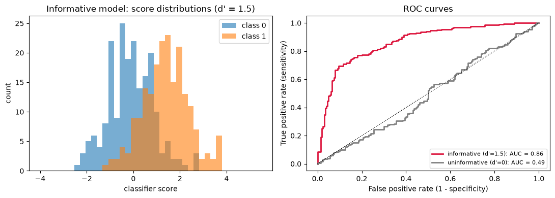
The uninformative model’s ROC hugs the diagonal (AUC ≈ 0.5): at every threshold, sensitivity gains are paid for one-to-one with false positives. The informative model bows toward the top-left corner. AUC is threshold-free and insensitive to class base rates, which makes it a standard headline metric for decoding models — though for clinical translation the operating point (a specific sensitivity/specificity pair) matters as much as the area (Chapter 41).
Wrap-up
Test error is U-shaped in complexity; training error is a biased, ever-improving illusion. Manage the bias–variance tradeoff, don’t ignore it.
Regularization turns complexity into a continuous dial: ridge shrinks smoothly, lasso sparsifies, elastic net blends the two — all deliberately trade a little bias for a big variance reduction.
Cross-validation is only as honest as its weakest step: any choice made with all the data (feature selection, scaling, tuning) leaks and inflates accuracy — dramatically, even on pure noise.
ROC/AUC characterize a classifier across all thresholds, separating discriminability from threshold choice.
Chapter 39 builds on this foundation: cross-validation schemes, nested CV for hyperparameter tuning, and unbiased performance estimation for predictive brain models.