AI and Neuroscience
Run this code: ⚡ In-browser lab · Colab · MATLAB Online
Overview
Artificial intelligence is a broad family of techniques for systems that perform complex, human-like tasks. It encompasses the machine learning of Chapters 37–40, but modern AI increasingly means something more specific: deep learning in multi-layer neural networks. Where classical ML models learn a single mapping from hand-designed features to an outcome, deep networks learn nonlinear, hierarchical re-representations of the raw data itself. Several properties follow. They can learn end-to-end, mapping raw input directly to output. They support transfer learning — representations learned on one task can be fine-tuned for another, which matters in neuroimaging where labeled data are scarce. And because they learn a representation of the joint distribution of features in a latent space, they can be generative, producing novel images or text. These ingredients combine in foundation models: very large networks trained by self-supervised learning on massive datasets (large language models like GPT are trained simply to predict the next word), which can then be adapted to many downstream tasks.
The building blocks are simple. A network node receives inputs from other nodes, weighted by connection strengths analogous to regression slopes, and passes the weighted sum through a nonlinear activation function (a sigmoid, tanh, or rectified linear unit). Nodes are organized in layers — input, hidden, and output — and in a feed-forward network information flows from data features through hidden layers to output nodes coding the prediction. A shallow network with linear activations implements something close to familiar models (logistic regression, or PCA-like dimensionality reduction); depth and nonlinearity are what add representational power. Networks learn gradually: a loss function quantifies prediction error, and backpropagation carries the gradient of that loss backward through the layers so each weight can be nudged downhill (gradient descent) across many passes through the data (epochs). Deep networks — two or more hidden layers — thereby learn features at increasingly abstract levels directly from raw data, instead of relying on features designed with domain knowledge.
Different architectures route information differently, and each major family brought a distinct advance. Convolutional neural networks (CNNs) slide learned filters across images, giving each unit a receptive field and producing feature maps that support translation-invariant recognition — reminiscent of convergent projections in visual cortex. Recurrent networks (RNNs) and their LSTM variants form directed cycles, giving them memory for sequential data such as speech or time series. Transformers replaced recurrence with self-attention, computing dependency scores between all elements of a sequence simultaneously; they are the engine of large language models. Generative families — GANs (a generator and discriminator trained adversarially), variational autoencoders (which compress data into a probabilistic latent space and reconstruct it), and diffusion models (which learn to reverse a gradual noising process) — can synthesize realistic new samples. Layered on top are training strategies: data augmentation, contrastive self-supervised learning, and transfer learning with fine-tuning, which together create an enormous space of model possibilities.
In neuroimaging, these tools are being used in three main ways. First, image processing and generation: CNNs and autoencoder architectures (e.g., U-Net) perform tumor and anatomical segmentation, registration, denoising, and accelerated image reconstruction, while generative models synthesize realistic brain images for data augmentation and “in silico” experiments. Second, decoding and prediction: deep models extend the neuromarker toolkit of Chapters 37–41. An AI-based speech decoder recently allowed a patient with ALS to communicate at 32 words per minute with 97% accuracy, sustained over months; “brain age” models trained on large structural datasets quantify the gap between predicted and chronological age, a marker linked to dementia, chronic pain, and mental health disorders. But deep learning does not always win: for behavioral prediction from resting-state connectivity, it has not reliably outperformed classical ML. Its biggest successes come where data are precise and richly structured — images, sounds, and language — and where samples are large. Third, and most provocative for cognitive neuroscience, artificial networks can serve as models of biological ones.
The logic of that third use is to treat an ANN as a simplified, testable model of neural computation and ask how deeply the correspondence runs. Correspondence can be tested at three levels: (1) does the network behave like humans, making the same kinds of errors? (2) do its internal tuning properties resemble neural ones? and (3) can its internal representations predict measured brain activity? For the third level, encoding models fit linear mappings from a layer’s unit activations (or their principal components) to voxel responses, testing generalization to held-out stimuli. Representational similarity analysis (RSA) takes a complementary, mapping-free approach: compute the matrix of pairwise (dis)similarities among stimuli in a network layer, do the same for the pattern of fMRI responses in a region, and correlate the two matrices. Two systems can share representational geometry even when no unit-to-voxel alignment exists. In a landmark study, Yamins and colleagues searched a large space of CNNs and found that the models best optimized for object recognition were also the best predictors of neural responses: top layers matched inferotemporal (IT) cortex and intermediate layers matched V4, at all three levels of correspondence (Figure 42.3). Performance-optimized networks, it seems, converge on representations resembling those the primate ventral stream evolved.
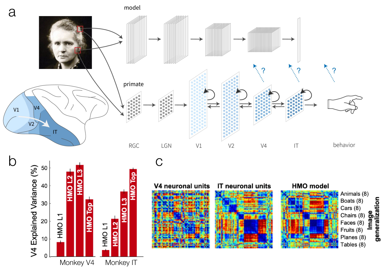
Artificial neural networks as models of brain function. (a) A CNN trained to recognize images can be compared, layer by layer, to the primate ventral visual hierarchy. (b) In a top-performing model, intermediate layers track macaque V4 neurons while the top layer tracks IT neurons. (c) Representational dissimilarity matrices across image categories: the model’s top layer reproduces the category structure seen in IT, but not V4. (Figure 42.3 from the book. © the authors and MIT Press; reproduced with permission — not covered by this site’s CC-BY license.)
Error-driven learning is another bridge between artificial and biological networks — and one you can hold in your hand mathematically. The Rescorla–Wagner model updates a value estimate from a prediction error, the mismatch between the reward received and the reward expected:
Vₜ — value (expected reward) on trial t · Rₜ — reward received on trial t (1 or 0) · δₜ — prediction error · α — learning rate (0–1)
where is the value (expected reward) on trial , the reward received (1 or 0), the prediction error, and the learning rate — how far each error moves the estimate.
Temporal difference (TD) learning generalizes this to sequences of states (the situation occupied at time step within a trial), where the error compares each moment’s prediction with the reward received plus the (discounted) prediction one step later:
δₜ — TD prediction error at time step t · rₜ — reward delivered at step t · V(sₜ) — value of the state occupied at step t · γ — temporal discount factor (0–1)
where is the reward delivered at time step , the value of the state occupied at step , the value of the next state, and the temporal discount factor that down-weights value one step in the future.
Phasic firing of midbrain dopamine neurons behaves strikingly like : unexpected rewards evoke bursts, fully predicted rewards evoke little response (the signal transfers to the earliest predictive cue), and omitted rewards produce dips below baseline. This correspondence — one of computational neuroscience’s success stories — underlies model-based fMRI, in which trial-by-trial model quantities like become parametric regressors (Chapter 20), and computational psychiatry, in which fitted parameters like characterize individuals and disorders. The same error-driven principle, scaled up, powers deep networks: reinforcement learning added to large language models trained on word prediction was a key ingredient of modern conversational AI.
The analogy has limits, and the field’s outstanding problems are instructive. Backpropagation, as implemented in AI, is not biologically plausible in its standard form, and brains learn from far less data than foundation models require. In both ANNs and cortex, single units have complex, entangled tuning — categories are “untangled” only at the population level, which is why multivariate pattern analyses (Chapters 37–41) are more informative than single voxels, and why individual-unit selectivity often fails to predict a unit’s importance to network performance. Practically, deep models remain hard to interpret (explainable-AI tools such as attention maps, saliency maps, LIME, and SHAP help, but only partially); they are prone to shortcut learning — exploiting confounds rather than the intended signal; they suffer domain shift when deployed on data unlike their training distribution; training frontier models costs tens of millions of dollars, concentrating capability; and algorithmic fairness must be engineered and audited, not assumed, before clinical use. These are exactly the generalization and validity issues of Chapters 39–41, now at larger scale — a reminder that the fundamentals of this book do not expire as models grow.
Hands-on tutorial
In this tutorial you will build, from scratch, the two computational ideas at the heart of this chapter: a prediction-error signal that behaves like phasic dopamine, and a representational similarity analysis comparing a small network’s layers to simulated brain regions. Everything runs with base numpy / base MATLAB — no deep learning toolboxes required.
Step 1 — Rescorla–Wagner prediction errors as a dopamine-like signal. We simulate conditioning: a cue predicts reward on 80% of trials, then reward stops (extinction). The prediction error drives learning — and traces out the classic dopamine pattern: large early bursts that shrink as learning proceeds, and negative dips when expected reward is omitted.
% Rescorla-Wagner learning
% Adapted from CANlab Computational Foundations course (github.com/canlab)
rng(0);                                % seed for reproducibility
alpha = 0.15;                          % alpha = learning rate (0-1)
n_trials = 120;                        % 80 acquisition + 40 extinction trials
r = double(rand(n_trials, 1) < 0.8);   % cue -> reward on 80% of trials
r(81:end) = 0;                         % extinction after trial 80

V = zeros(n_trials + 1, 1); pe = zeros(n_trials, 1);
for t = 1:n_trials
    pe(t) = r(t) - V(t);               % prediction error (dopamine-like)
    V(t+1) = V(t) + alpha * pe(t);     % value update
end

figure;
subplot(1,2,1); plot(V, 'LineWidth', 2); title('Learned value V'); xlabel('Trial');
subplot(1,2,2); plot(pe); title('Prediction error \delta'); xlabel('Trial');
import numpy as np
import matplotlib.pyplot as plt
rng = np.random.default_rng(0) # seed for reproducibility
alpha, n_trials = 0.15, 120 # alpha = learning rate; 80 acquisition + 40 extinction trials
r = (rng.random(n_trials) < 0.8).astype(float) # cue -> reward on 80% of trials
r[80:] = 0.0 # extinction after trial 80
V = np.zeros(n_trials + 1)
pe = np.zeros(n_trials)
for t in range(n_trials):
pe[t] = r[t] - V[t] # prediction error (dopamine-like)
V[t + 1] = V[t] + alpha * pe[t] # value update
fig, ax = plt.subplots(1, 2, figsize=(9, 3))
ax[0].plot(V); ax[0].set(title="Learned value V", xlabel="Trial")
ax[1].plot(pe); ax[1].set(title="Prediction error $\\delta$", xlabel="Trial")Example output:
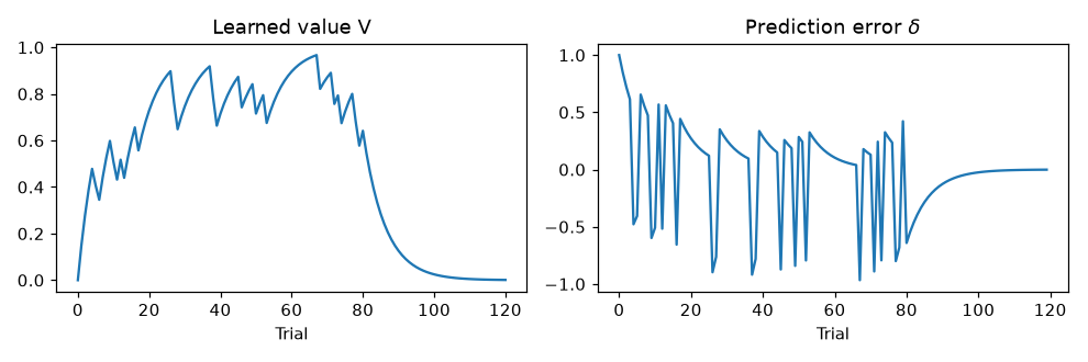
Value climbs toward the true reward rate (0.8), then extinguishes after trial 80; prediction errors are large early in acquisition, shrink as learning proceeds, and dip negative when expected reward is omitted.
Step 2 — Toy representational similarity analysis. We create stimuli from four categories, pass them through a network layer, simulate a category-coding “brain region,” and ask whether the two share representational geometry by correlating their representational dissimilarity matrices (RDMs) — the same logic as Figure 42.3c.
% Toy RSA: does a model layer's geometry match a brain region's?
n_stim = 32; n_feat = 20;                       % 32 stimuli, 20 features each
categ = repelem(1:4, 8)';                       % 4 categories x 8 exemplars
protos = randn(4, n_feat);                      % category prototype patterns
X = protos(categ, :) + 0.8 * randn(n_stim, n_feat);   % stimulus features

layer = max(X * randn(n_feat, 10), 0);          % random ReLU layer
brain = protos(categ, :) * randn(n_feat, 50) ...
        + 2 * randn(n_stim, 50);                % category-coding "region"

rdm_layer = 1 - corr(layer');                   % correlation-distance RDMs
rdm_brain = 1 - corr(brain');
iu = find(triu(ones(n_stim), 1));               % off-diagonal entries
rho = corr(rdm_layer(iu), rdm_brain(iu), 'type', 'Spearman');
fprintf('Model-brain RDM correlation: rho = %.2f\n', rho);
from scipy.stats import spearmanr
n_stim, n_feat = 32, 20 # 32 stimuli, 20 features each
categ = np.repeat(np.arange(4), 8) # 4 categories x 8 exemplars
protos = rng.standard_normal((4, n_feat)) # category prototype patterns
X = protos[categ] + 0.8 * rng.standard_normal((n_stim, n_feat)) # prototype + exemplar noise
layer = np.maximum(X @ rng.standard_normal((n_feat, 10)), 0) # random ReLU layer
brain = (protos[categ] @ rng.standard_normal((n_feat, 50))
+ 2 * rng.standard_normal((n_stim, 50))) # category-coding "region"
def rdm(A): # correlation-distance RDM
return 1 - np.corrcoef(A)
iu = np.triu_indices(n_stim, k=1) # off-diagonal entries
rho = spearmanr(rdm(layer)[iu], rdm(brain)[iu]).statistic
print(f"Model-brain RDM correlation: rho = {rho:.2f}")Example output:
Model-brain RDM correlation: rho = 0.34Even this random (untrained) ReLU layer shares some geometry with the category-coding region, because the category signal in the stimuli leaks through the projection — the labs show how training strengthens this correspondence, and how an untrained layer instead best matches an early sensory region.
The full labs go further: temporal difference learning that reproduces the transfer of the dopamine burst from reward to cue (and the omission dip), the effect of the learning rate on value trajectories, and — for RSA — a tiny multilayer network trained by backpropagation in pure numpy/MATLAB, showing that training for a task is what makes a layer’s geometry brain-like, exactly the logic of the Yamins experiment.
Open the full Python lab notebook → or download the MATLAB live script, which mirrors it.


Thought questions
A CNN’s top layer predicts IT responses and reproduces IT’s representational geometry. What further evidence would you require before calling the CNN a model of IT computation, rather than merely a system correlated with it? Consider the three levels of correspondence, causal manipulations, and what “same computation, different substrate” would even mean.
The dopamine–TD correspondence is celebrated, yet backpropagation — the learning rule that makes deep networks work — has no accepted biological implementation, and humans learn language from orders of magnitude less data than an LLM. Where exactly do you place the boundary between “the brain does something like this” and “this is an engineering trick”? What experiment could move that boundary?
LLM embeddings predict fMRI responses to natural language remarkably well. Does this tell us the brain predicts upcoming words, that both systems track the statistics of language, or only that both compress the same input? Design an analysis that could distinguish these interpretations — and note which of them RSA alone could never settle.
Imagine building a foundation model for fMRI: what would the training corpus be, what self-supervised objective would you use, and which of the chapter’s outstanding issues (shortcut learning, domain shift, interpretability, fairness) do you think would bite hardest when the model is fine-tuned as a clinical neuromarker?
In both ANNs and cortex, single units are entangled and category structure lives at the population level. If cognition is best described by architectures, learning rules, and objective functions rather than by box-and-arrow modules, what happens to classical cognitive-neuroscience constructs like “the face area” or “working memory”? Argue for or against the reframing.
Quiz yourself
Q1. What distinguishes deep learning from the classical machine learning models of Chapters 37–41?
Answer: Deep learning uses multi-layer neural networks that learn hierarchical, usually nonlinear re-representations of the raw data, rather than fitting a single mapping from hand-designed features to an outcome. This enables end-to-end learning, transfer learning, and generative modeling.
Q2. What does a single node in a neural network compute, and why is the activation function important?
Answer: A node takes a weighted sum of its inputs (weights are analogous to regression slopes) and passes it through an activation function such as a sigmoid, tanh, or ReLU. The nonlinearity of the activation function is what lets networks capture complex relationships that linear models cannot.
Q3. What is a foundation model, and what training approach makes it possible?
Answer: A foundation model is a very large network trained on massive datasets using self-supervised learning (e.g., predicting the next word or a masked portion of the input), which can then be adapted or fine-tuned for many downstream tasks. Large language models like GPT are the canonical example.
Q4. In the Rescorla–Wagner model, what is the prediction error, and how does the learning rate shape learning?
Answer: The prediction error is , the difference between the reward received and the reward expected; the value estimate is updated by . With small , learning is slow but stable; with large , the value tracks recent outcomes quickly but noisily ( means expectation simply equals the last reward).
Q5. Describe the three signatures of phasic dopamine firing that match the TD prediction error.
Answer: (1) Unexpected rewards evoke a burst; (2) once a cue reliably predicts reward, the burst transfers to the cue and the predicted reward itself evokes little response; (3) omission of a predicted reward produces a dip below baseline firing at the expected time — a negative prediction error.
Q6. What is a representational dissimilarity matrix (RDM), and why does comparing RDMs let us relate a network layer to a brain region without mapping units to voxels?
Answer: An RDM is the matrix of pairwise dissimilarities (e.g., 1 − correlation) among the response patterns evoked by a set of stimuli. Because it characterizes the geometry of a representation rather than its coordinates, two systems with entirely different units can be compared by correlating their RDMs — a second-order comparison.
Q7. What did Yamins and colleagues find when they compared many CNNs to neurons in the primate ventral stream?
Answer: CNNs optimized for object-recognition performance best predicted neural responses: their top layers matched IT cortex and intermediate layers matched V4, in encoding-model fits and RDM comparisons alike. This suggests the ventral stream’s representations resemble those of networks optimized for the same task.
Q8. Name three outstanding issues that limit the deployment of deep learning models as clinical neuromarkers, and one emerging remedy for each.
Answer: Interpretability — addressed partially by explainable-AI tools (saliency maps, attention visualization, LIME/SHAP); shortcut learning on confounds — mitigated by data augmentation, synthetic data, and adversarial training; and domain shift across scanners or populations — addressed by fine-tuning and augmentation in the new domain. (Cost of training and algorithmic fairness are also acceptable answers.)
 The book: Elements of Functional Magnetic Resonance Imaging — Wager & Lindquist, MIT Press