Applying Predictive Models to fMRI Data
Run this code: ⚡ In-browser lab · Colab · MATLAB Online
Overview
Previous chapters covered the algorithms used in predictive modeling (Chapter 38) and how to train and test models without fooling yourself (Chapter 39). This chapter steps back to the design choices that shape what a predictive model is and what it can be used for. There are many: which outcome to predict and which sources of variation to model, which type of brain data to use, whether to fit one model per person or one model for the population, how much of the brain to include, and how to construct and embed features. Prediction error is usually the first criterion for judging a model, but it is not the only one — sensitivity and specificity, reproducibility, generalizability to new populations and tasks, robustness to noise, and interpretability all matter, especially when models are meant to become reusable measures.
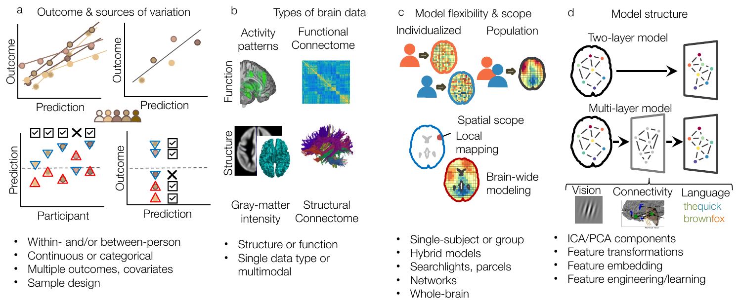
Varieties of predictive models using MRI and fMRI data. Key choices include (a) the outcome(s) and sources of variation modeled — within-person and/or between-person, continuous or categorical; (b) the type of brain data used; (c) the model’s flexibility and spatial scope, from individualized to population-level and from local to whole-brain; and (d) model construction and feature embedding. (Figure 40.1 from the book. © the authors and MIT Press; reproduced with permission — not covered by this site’s CC-BY license.)
A first choice is the outcome and the sources of variation it reflects. Within-person predictions — decoding which stimulus was shown on a trial, or how much pain a person felt from moment to moment — are typically much stronger than between-person predictions of individual differences, because mind–brain relationships within an individual carry far fewer sources of error. Between-person models must contend with individual differences in head movement, vascular health, and medication on the brain side, and with rating-scale usage, decision biases, and outcome unreliability on the psychological side. Within-person models also make a weaker measurement demand: they require only that a person’s reports be self-consistent (a “6” hurts more than their own “5”), not that scales be calibrated across people. Outcomes can be continuous or categorical, and although two-class classification has been the most common approach, artificially binarizing continuous scores (especially by median split) introduces error and bias, and two-class designs carry minimal information about outcome variation — making them particularly vulnerable to confounds.
That vulnerability arises because machine learning models are “greedy”: they exploit all information correlated with the outcome labels, including confounding processes that are conceptually distinct from the target. A classifier trained to separate painful from non-painful conditions will happily use activity related to arousal and attention. The most powerful remedy is sample design: include diverse examples of confusable processes (aversive images, sounds) with “no pain” labels to force specificity, and include multiple variants of the target construct (different types of painful stimuli) to force the model toward generalizable representations rather than idiosyncrasies of one stimulus type.
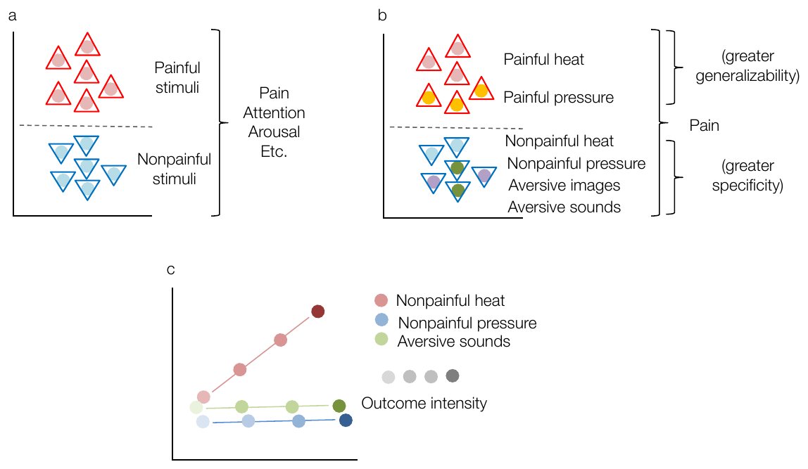
Sample design. (a) Two-class classification with only two task conditions is especially subject to confounding by attention, arousal, and other correlated processes. (b) Including more diverse “control” examples increases specificity to the target construct, and including diverse examples of the construct increases generalizability. (c) A regression version in which target and control conditions vary along an intensity continuum. (Figure 40.2 from the book. © the authors and MIT Press; reproduced with permission — not covered by this site’s CC-BY license.)
The type of brain data matters too. Structural measures (gray matter volume, cortical thickness) are highly reliable (often > 0.9) and suited to stable traits that change slowly; task fMRI is suited to states that vary within person across seconds. Reliability of resting-state connectivity in individual regions is low (generally < 0.4), though multivariate patterns can be far more reliable (> 0.8) with enough data per person. Beyond reliability, predictive power requires a strong true brain–outcome link: brain structure predicts outcomes with gross anatomical consequences (dementia, age) well, but appears to be a poor predictor of many cognitive and mental-health phenotypes. Brain data predict best when they are both reliable and directly relevant to the outcome.
The level of analysis is a choice between individualized models — trained within a single person, sensitive to fine-grained idiosyncratic topography, but applicable only to that person — and population-level models that capture topography conserved across individuals. Population-level models have three big advantages for cumulative science: they are true predictive models that can be applied prospectively to new individuals and datasets; they are less susceptible to confounds, because the model is less flexible and participant-specific confounds tend to average out; and they support group inference on the model weights themselves, connecting patterns to converging evidence from other methods. Hybrids such as group-regularized individual prediction (GRIP) weight population-level and individual predictions by their relative reliability and can outperform both.
Spatial scope ranges from single regions of interest, through searchlight and parcel-wise “information mapping” — thousands of local multivariate models, each summarized by its local accuracy — to a single integrated model spanning the whole brain. Searchlights identify where predictive information lives but cannot capture patterns distributed across systems, require multiple-comparisons correction, and invite inflated post-hoc accuracy estimates. Whole-brain predictive maps integrate all measures into one model whose overall performance can be validated prospectively; regularization, dimension reduction, and kernel methods keep such maps stable even when voxels far outnumber observations.
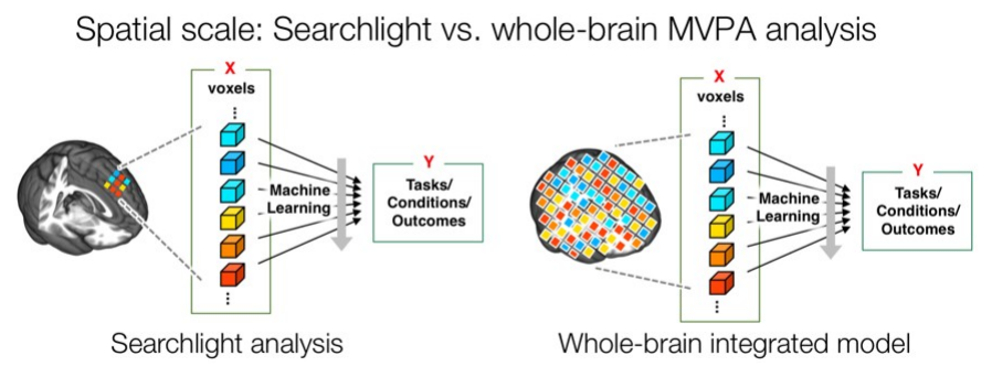
Two spatial scopes for multivariate analysis. A searchlight analysis (left) tests thousands of local predictive models to map areas that predict above chance. A whole-brain predictive map (right) builds one integrated model across regions, which can be tested prospectively on new datasets. (Figure 40.3 from the book. © the authors and MIT Press; reproduced with permission — not covered by this site’s CC-BY license.)
Finally, model structure and feature embedding determine what the model’s inputs mean. Feature engineering, rescaling, and dimension reduction (e.g., PCA) can be viewed as intermediate layers between input data and predicted outcomes — a framing that connects classical machine learning to deep networks (Chapter 42). Embedding brain activity in feature spaces defined by receptive-field properties, action concepts, or language models enables encoding–decoding models that can reconstruct seen images, predict responses to novel words, and even decode dream content. For neuroscientific inference, linear mappings between psychological features and brain responses are key: if features can be read out only through a complex nonlinear function, the brain cannot really be said to represent them.
From model to measure. Once a population-level model is trained, applying it to new data is remarkably simple. The model is a fixed weight map (a “signature”), and its response to a new brain image is a weighted average — the dot product:
r — pattern response (signature score for one image) · w — fixed signature weights (voxels × 1) · x — new brain image as a vector (voxels × 1) · wᵥ, xᵥ — weight and image value at voxel v · V — number of voxels
where is the pattern response (the signature’s score for the image), the fixed vector of signature weights (one per voxel), the new brain image arranged as a vector, and their values at voxel , and the number of voxels.
This generalizes the region-of-interest average: an ROI mask of 1’s and 0’s yields the average signal (up to scaling), whereas a pattern weights each voxel by its trained contribution. Scale-free variants divide out image magnitude: cosine similarity, — where is the angle between the weight and image vectors and the vector norm (overall magnitude) — is invariant to multiplicative rescaling of the image, and Pearson correlation — cosine similarity after mean-centering both vectors — is additionally invariant to uniform additive shifts. These invariances matter for calibration when images come from different scanners or protocols: raw dot products can shift dramatically with scanner gain, while within-person comparisons and correlation-based metrics are far more stable. Performance on new data is then quantified with paired forced-choice tests (which condition has the higher response, within person — baseline differences cancel), and with ROC curves, sensitivity, and specificity for single-interval classification. This machinery — fixed weights, pattern responses, forced-choice and ROC tests — is exactly how signatures such as the Neurologic Pain Signature are applied and validated, and it sets up the treatment of neuromarkers in Chapter 41.
Hands-on tutorial
In this tutorial you will apply a fixed, pretrained pattern to new condition images and quantify its performance. The MATLAB tabs use CANlab tools and real signatures; the Python tabs mirror the logic with a simulated signature so everything runs in your browser.
Step 1 — Compute pattern responses on new images. The pattern response is a dot product between the signature weights and each image; correlation and cosine similarity are scale-free alternatives.
% Requires CanlabCore + Neuroimaging_Pattern_Masks + SPM12 on your path
% Adapted from CANlab tutorial canlab_help_9 (github.com/canlab)
test_data = load_image_set('emotionreg');       % 30 subjects, [regulate - look]
[pats, patnames] = load_image_set('pain_cog_emo');  % library of published pain/cognition/emotion patterns
sig = get_wh_image(pats, 8);                    % whole-brain pain pattern (Kragel 2018)

% Pattern response = weighted sum (dot product) of image values and weights
pexp = apply_mask(test_data, sig, 'pattern_expression', 'ignore_missing');

% Scale-free alternatives: correlation and cosine similarity
pexp_r   = apply_mask(test_data, sig, 'pattern_expression', 'ignore_missing', 'correlation');
pexp_cos = apply_mask(test_data, sig, 'pattern_expression', 'ignore_missing', 'cosine_similarity');
import numpy as np
import matplotlib.pyplot as plt
rng = np.random.default_rng(0) # seed, for reproducibility
n_vox, n_sub = 2000, 30 # n_vox = "voxels", n_sub = new test subjects
w = rng.standard_normal(n_vox) * (rng.random(n_vox) < 0.10) # FIXED signature weights (~10% of voxels nonzero)
# New subjects' condition images: the target condition expresses the signature
amp = rng.normal(1.0, 0.4, n_sub) # per-subject expression strength (mean 1.0, SD 0.4)
pain = amp[:, None] * w + 3 * rng.standard_normal((n_sub, n_vox)) # 3 = voxel noise SD
warm = 3 * rng.standard_normal((n_sub, n_vox)) # control condition: noise only, no signature
resp_pain, resp_warm = pain @ w, warm @ w # pattern response = dot product
def corr_with_pattern(X, w): # scale-free alternative (Pearson r)
Xc, wc = X - X.mean(1, keepdims=True), w - w.mean()
return (Xc @ wc) / (np.linalg.norm(Xc, axis=1) * np.linalg.norm(wc))
print(f"mean pattern response: pain = {resp_pain.mean():.1f}, warmth = {resp_warm.mean():.1f}")
print(f"mean correlation with pattern: pain = {corr_with_pattern(pain, w).mean():.2f}, "
f"warmth = {corr_with_pattern(warm, w).mean():.2f}")
plt.figure(figsize=(4.6, 3.4)) # paired responses, one line per subject
plt.plot([0, 1], np.c_[resp_pain, resp_warm].T, "-o", color="gray", alpha=0.4)
plt.xticks([0, 1], ["pain", "warmth"]); plt.ylabel(r"pattern response $w^\top x$")
plt.title("Signature responses on new subjects")
plt.tight_layout()Example output:
mean pattern response: pain = 171.2, warmth = -1.5
mean correlation with pattern: pain = 0.09, warmth = -0.00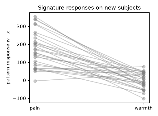
Pattern responses on 30 new subjects: the pain condition expresses the signature strongly for nearly every subject, while the warmth control hovers near zero. Note the small mean correlation (≈ 0.09): with 2,000 noisy voxels, even a strongly expressed signature explains a small fraction of image variance — the response is reliable because it pools over many voxels.
Step 2 — Test performance: forced choice and ROC. In a paired forced-choice test we ask, for each subject, which condition produced the larger response — subject-level baseline shifts cancel. ROC analysis characterizes single-interval classification across thresholds.
% Simulated paired responses for 30 subjects (or use pexp values from real data)
rng(1); n = 30;                           % seed, for reproducibility; n = subjects
resp_pain = 1.0 + 0.5 * randn(n, 1);      % signature response, target condition
resp_warm = 0.0 + 0.5 * randn(n, 1);      % signature response, control condition

acc_fc = mean(resp_pain > resp_warm)      % paired forced-choice accuracy

% CanlabCore roc_plot: single-interval, then paired forced-choice
ROC  = roc_plot([resp_pain; resp_warm], [true(n,1); false(n,1)]);
ROC2 = roc_plot([resp_pain; resp_warm], [true(n,1); false(n,1)], 'twochoice');
from sklearn.metrics import roc_curve, roc_auc_score
acc_fc = np.mean(resp_pain > resp_warm) # paired forced-choice accuracy
y = np.r_[np.ones(n_sub), np.zeros(n_sub)] # labels: 1 = pain, 0 = warmth
val = np.r_[resp_pain, resp_warm] # one threshold across all images
fpr, tpr, thr = roc_curve(y, val)
j = np.argmax(tpr - fpr) # Youden's J: best balanced threshold
print(f"forced-choice acc = {acc_fc:.2f}, AUC = {roc_auc_score(y, val):.2f}, "
f"sensitivity = {tpr[j]:.2f}, specificity = {1 - fpr[j]:.2f}")
plt.figure(figsize=(3.8, 3.6)) # single-interval ROC curve
plt.plot(fpr, tpr, "-", color="tab:blue"); plt.plot([0, 1], [0, 1], "k:", lw=1)
plt.plot(fpr[j], tpr[j], "o", color="tab:blue") # marks the best balanced threshold
plt.xlabel("1 - specificity"); plt.ylabel("sensitivity"); plt.title("Single-interval ROC")
plt.tight_layout()Example output:
forced-choice acc = 0.93, AUC = 0.98, sensitivity = 0.93, specificity = 0.97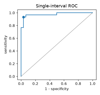
The single-interval ROC curve (AUC = 0.98). The dot marks the best balanced threshold (Youden’s J): sensitivity 0.93, specificity 0.97. Forced-choice accuracy (0.93) needs no threshold at all — each subject’s baseline cancels in the paired comparison.
The full labs go further: they build a signature with spatially structured weights, apply it to three conditions (target, confusable control, and neutral control) to probe specificity, and show how scanner gain and offset distort raw dot products but not correlation-based metrics or within-person forced-choice tests.
Open the full Python lab notebook → or download the MATLAB live script, which mirrors it using CANlab tools.


Thought questions
A team proposes to classify depressed vs. non-depressed adolescents from resting-state connectivity; another proposes to predict moment-to-moment sadness within individuals watching films. Using the concepts of sources of variation, measurement reliability, and the absolute-scale requirement, compare the expected effect sizes and the meaning of success in each project.
You are designing the training study for an “anxiety signature.” Applying the sample-design principles of Figure 40.2, what target and control conditions would you include to maximize specificity (against general negative affect and arousal) and generalizability (across kinds of anxiety), and what would you deliberately vary along a continuum?
For (a) testing whether object identity is encoded in a person’s lateral occipital cortex, and (b) providing an outcome measure for a multi-site analgesic clinical trial, argue for an individualized or a population-level model — considering confound robustness, open-ended specificity testing, and applicability to new people.
A colleague reports 62% decoding accuracy in a searchlight analysis and interprets the peak searchlight as the region that “encodes” the process. What inferential problems arise from testing thousands of local models and selecting the best, and how does building one integrated whole-brain model, tested prospectively, change what can be claimed?
Your signature’s raw pattern responses are, on average, twice as large at Site B as at Site A, yet within-site condition differences are similar. Which analyses remain valid without any harmonization, which metrics (dot product, cosine, correlation) would you choose for cross-site comparisons, and when would you need explicit recalibration?
Quiz yourself
Q1. What is a “pattern response,” and how does it relate to a classic ROI average?
Answer: The pattern response is the dot product between a fixed weight map and a brain image, — a weighted average of image values with weights given by the pattern. If the pattern is a mask of 1’s and 0’s, it reduces (up to scaling) to the ordinary ROI average.
Q2. Why are within-person predictions typically stronger than between-person predictions of individual differences?
Answer: Within-person relationships avoid many irreducible error sources that affect between-person comparisons — individual differences in head motion, vasculature, and medication on the brain side, and rating-scale usage, biases, and outcome unreliability on the psychological side. Within-person models also require only self-consistency of reports, not that scales be calibrated identically across people.
Q3. What is wrong with median-splitting a continuous outcome to make a two-class classification problem?
Answer: Binarizing continuous scores discards information about outcome variation, introducing error and bias that reduce power and validity. Two-class outcomes also make models more vulnerable to confounds and floor/ceiling effects, whereas multi-level outcomes let you evaluate sensitivity across a dynamic range.
Q4. Machine learning models are “greedy.” What does that mean, and what sample-design strategy mitigates the resulting confounding?
Answer: Models use all information correlated with the outcome labels, including confounds like arousal and attention that are conceptually distinct from the target. The remedy is to include diverse confusable processes with control labels (forcing specificity) and multiple variants of the target construct (forcing generalizable representations), and to balance labels on covariates.
Q5. Contrast a searchlight analysis with a whole-brain predictive map.
Answer: A searchlight fits thousands of local multivariate models, saving each one’s accuracy at its center voxel to map where information lives; it misses patterns distributed across systems, requires multiple-comparisons correction, and inflates post-hoc accuracy. A whole-brain map is one integrated model across regions whose overall performance can be tested prospectively on new data.
Q6. Which pattern-similarity metrics are invariant to multiplicative scanner gain, and which are also invariant to a uniform additive offset in the image?
Answer: Cosine similarity is invariant to multiplicative rescaling of the image, because the image’s norm is divided out. Pearson correlation — cosine similarity after mean-centering — is invariant to both multiplicative gain and uniform additive offsets. The raw dot product is sensitive to both.
Q7. Why does paired forced-choice accuracy usually exceed single-interval classification accuracy for the same data?
Answer: In a forced-choice test each subject serves as their own baseline: we only ask which of two conditions produces the higher response, so between-subject differences in overall signal level cancel out. Single-interval classification must place one threshold across all subjects, so between-subject baseline variance counts against it.
Q8. Name three criteria (beyond raw accuracy) for a good predictive model.
Answer: Any three of: it makes quantitative, falsifiable predictions; it predicts outcomes outside the brain (behavior, experience, clinical status); it can easily be tested prospectively on new datasets; it is simple to interpret; it is only as complex as it needs to be; and it is not over-interpreted as a complete or uniquely “correct” explanation.
 The book: Elements of Functional Magnetic Resonance Imaging — Wager & Lindquist, MIT Press