Machine Learning Principles and Algorithms
Run this code: ⚡ In-browser lab · Colab · MATLAB Online
Overview
Most predictive brain models draw on machine learning, a discipline at the intersection of computer science and statistics. Machine learning is a large umbrella of techniques. Supervised learning algorithms optimize prediction of known outcomes from labeled data — regression when the outcome is continuous, classification when it is categorical. Unsupervised algorithms instead group unlabeled data into clusters or coherent components (clustering, PCA, ICA; see Chapter 31). In neuroimaging, the observations are often participants or trials, the features () are voxels, connections, or graph metrics, and the outcome () might be patient status, stimulus category, or a continuous symptom score.
One useful way to understand machine learning is as a set of variations on classical statistical models. The goal is to learn a function that accurately predicts ; multiple linear regression is the special case , where is a vector of feature weights and a scalar intercept (the bias), with weights estimated by minimizing a loss function. Machine learning is flexible about how that loss is defined. A general and enormously influential form adds a regularization (penalty) term to the measure of fit:
𝓛(w) — total loss to minimize · w — model weights · E(w) — data-fit term (e.g., sum of squared errors) · R(w) — regularization penalty encoding prior constraints · λ — hyperparameter weighting fit vs. penalty
where is the vector of model weights, a measure of fit (e.g., the sum of squared errors), a regularization penalty that builds in prior knowledge and constraints (e.g., a preference for small or sparse weights), and the hyperparameter controls their relative contribution.
Other algorithms swap the fit term itself — support vector machines use a hinge loss, and absolute-error losses resist influential data points better than squared error.
The deepest difference from classical statistics is the explicit focus on generalizability. In classical regression, error is evaluated on the same data used for fitting, so adding parameters always improves apparent fit — and if the number of features reaches the number of observations (), a linear model can fit any dataset perfectly, with zero error, without capturing anything that generalizes. This is overfitting: the model absorbs noise idiosyncratic to the sample. The machine learning remedy is to partition data into independent training and test sets. Even a wildly overfit model can then be fairly evaluated on held-out data, and models of different complexity — including non-nested models with different structures — can be compared on equal footing. Cross-validation (Chapter 39) systematizes this within a single dataset, and is typically followed by validation on fully independent data.
Complexity itself trades off two sources of error. Simple models underfit: they are systematically wrong in the same way in every sample (high bias). Complex models fit the training data beautifully but change drastically from sample to sample (high variance). Expected prediction error on new data decomposes, approximately, into , so test error follows a characteristic U-shaped curve as complexity grows — falling while added flexibility captures real structure, then rising as the model begins to memorize noise. Training error, by contrast, only decreases. Regularization, ensemble averaging (bagging, boosting, random forests), and dimension reduction are all ways of managing this tradeoff — accepting a little bias to buy a large reduction in variance.
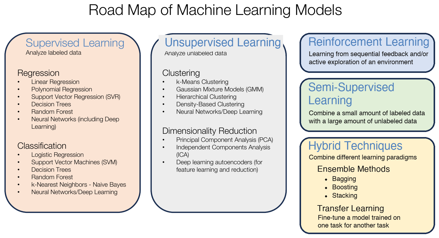
A roadmap of commonly used machine learning models, organized into five major groups: supervised learning, unsupervised learning, reinforcement learning, semi-supervised learning, and hybrid techniques (ensemble methods and transfer learning). fMRI prediction pipelines often combine unsupervised data reduction with supervised prediction. (Figure 38.2 from the book. © the authors and MIT Press; reproduced with permission — not covered by this site’s CC-BY license.)
Classification algorithms use an object’s features to decide which class it belongs to. A binary linear classifier computes a score and predicts class +1 when and -1 otherwise. Geometrically, and the bias define a hyperplane that splits feature space in two; algorithms differ in how they place it. Linear discriminant analysis maximizes between-class relative to within-class variance under normality assumptions; logistic regression models the log odds of class membership, yielding calibrated probabilities. The support vector machine (SVM) chooses the hyperplane with the largest margin — the greatest distance to the nearest training points, which are called the support vectors because they alone determine the solution. When classes overlap, slack variables measure each point’s degree of misclassification, and the objective becomes
w — hyperplane weight vector · b — bias (threshold) · ‖w‖² — inversely related to margin width · ξᵢ — slack: degree of misclassification of point i · C — margin-vs-errors tradeoff hyperparameter · n — number of training points
where and define the hyperplane, is inversely related to the margin width, is the slack (degree of misclassification) for training point , the number of training points, and the hyperparameter trades off margin width against training errors.
SVMs are accurate, fast, and stable with very large numbers of features — one reason for their popularity in fMRI, where kernels map the data into an similarity space so computation scales with observations rather than voxels. Simple nonlinear alternatives include -nearest neighbors (majority vote among the most similar training examples) and naive Bayes (combining per-feature class probabilities under an independence assumption — often unrealistic, yet remarkably effective when features are many and examples few).
Regression algorithms predict continuous outcomes, and here regularization does the heavy lifting in high dimensions. The two most common penalties are L1 and L2:
R_L1 — lasso penalty (sum of absolute weights) · R_L2 — ridge penalty (sum of squared weights) · w_j — weight on feature j · p — number of features
where is the weight on feature and the number of features; each penalty enters the loss as with regularization strength .
L2 regularization defines ridge regression: all coefficients shrink smoothly toward zero, stabilizing estimates when predictors are highly multicollinear — but none become exactly zero, so every feature stays in the model. L1 regularization defines the LASSO: as grows, coefficients of the least important features hit exactly zero, producing a sparse model. Sparsity is attractive for simple measurement models, but applied directly to brain voxels it tends to pick one arbitrary representative from each set of correlated voxels, scattering “speckles” of predictive features across the brain. Structured variants (group LASSO, fused LASSO, GraphNet) constrain selection to spatially coherent sets; the elastic net combines both penalties and behaves better than LASSO with correlated features; and LASSO-PCR applies sparsity to principal-component scores rather than voxels, selecting distributed components instead of isolated speckles. Shrinkage deliberately introduces bias — the training-data fit is no longer optimal — in exchange for lower variance: more stable, more reproducible, and often more accurate weights in new data.
Beyond these workhorses, decision trees segment feature space into regions with distinct predicted values (nonparametric, nonlinear, fast), and random forests average many trees trained on random subsamples. Ensemble strategies — bagging, boosting, stochastic gradient descent, dropout — build robustness by averaging over stochastically perturbed models. Extensions such as partial least squares (PLS) and canonical correlation analysis (CCA) decode multiple outcomes simultaneously by finding maximally covarying latent components of brain and behavior; encoding–decoding models predict each voxel’s activity from rich stimulus feature spaces and then invert the mapping; and deep neural networks learn hierarchies of intermediate features directly from data (Chapter 42). Whatever the algorithm, the principles above are constant: define a loss, control complexity, and evaluate on data the model has never seen.
Hands-on tutorial
These exercises make the chapter’s two central lessons concrete with simulated data: (1) test error is U-shaped in model complexity, and (2) any data-dependent choice made outside cross-validation poisons the estimate of accuracy. The full labs extend both, adding lasso vs. ridge coefficient paths and ROC curves.
Step 1 — Overfitting and the U-shaped test error curve. We fit polynomials of increasing degree to noisy data from a smooth true function. Training error always falls; test error falls, bottoms out near the true complexity, then rises.
% Requires only base MATLAB
rng(1);                                     % seed for reproducibility
f = @(x) sin(2*x);                          % true function
xtr = 4*rand(30,1); ytr = f(xtr) + .4*randn(30,1);   % training set: 30 points, noise SD = 0.4
xte = 4*rand(200,1); yte = f(xte) + .4*randn(200,1); % test set: 200 independent points

degrees = 1:12;                             % complexity levels to sweep
for d = degrees
    p = polyfit(xtr, ytr, d);               % fit on training data only
    train_mse(d) = mean((ytr - polyval(p, xtr)).^2);
    test_mse(d)  = mean((yte - polyval(p, xte)).^2);
end

figure; plot(degrees, train_mse, 'b.-', degrees, test_mse, 'r.-');
set(gca, 'YScale', 'log');                  % log scale keeps the U-shape visible
legend({'Training error' 'Test error'});
xlabel('Polynomial degree (model complexity)'); ylabel('MSE (log scale)');
import numpy as np, matplotlib.pyplot as plt
rng = np.random.default_rng(1) # seed for reproducibility
f = lambda x: np.sin(2 * x) # true function
xtr = 4 * rng.random(30); ytr = f(xtr) + .4 * rng.standard_normal(30) # training set: 30 points, noise SD = 0.4
xte = 4 * rng.random(200); yte = f(xte) + .4 * rng.standard_normal(200) # test set: 200 independent points
degrees = np.arange(1, 13) # complexity levels to sweep
train_mse, test_mse = [], []
for d in degrees:
p = np.polyfit(xtr, ytr, d) # fit on training data only
train_mse.append(np.mean((ytr - np.polyval(p, xtr)) ** 2))
test_mse.append(np.mean((yte - np.polyval(p, xte)) ** 2))
plt.plot(degrees, train_mse, "b.-", label="Training error")
plt.plot(degrees, test_mse, "r.-", label="Test error")
plt.yscale("log") # log scale keeps the U-shape visible
plt.xlabel("Polynomial degree (model complexity)"); plt.ylabel("MSE (log scale)")
plt.legend()Example output:
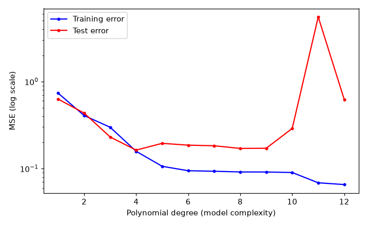
Training error (blue) only falls as degree grows. Test error (red) bottoms out near degree 4 — close to the true smooth function — then climbs and finally explodes as high-degree polynomials chase noise.
Step 2 — Cross-validation done wrong vs. right. The features here are pure noise — there is nothing to find. Selecting the most outcome-correlated features on the full dataset before cross-validating leaks test information into training and yields impressively wrong accuracy; selecting inside each fold gives the honest answer (~50%).
rng(7);                     % seed for reproducibility
n = 50; p = 2000; k = 20;   % n = participants, p = noise features, k = features to select
X = randn(n, p); y = [ones(n/2,1); -ones(n/2,1)];  % features are pure noise

% WRONG: select features using ALL data, then cross-validate
r = corr(X, y); [~, sel] = maxk(abs(r), k);
acc_wrong = 1 - crossval('mcr', X(:, sel), y, ...
    'Predfun', @(xt,yt,xv) sign(xv * (xt \ yt)), 'KFold', 10);

% RIGHT: feature selection re-done inside every training fold
cv = cvpartition(n, 'KFold', 10); correct = 0;
for i = 1:cv.NumTestSets
    tr = training(cv, i); te = test(cv, i);
    r = corr(X(tr,:), y(tr)); [~, sel] = maxk(abs(r), k);
    yhat = sign(X(te, sel) * (X(tr, sel) \ y(tr)));
    correct = correct + sum(yhat == y(te));
end
acc_right = correct / n;
fprintf('Wrong CV: %.0f%%  Right CV: %.0f%%  (chance = 50%%)\n', ...
    100*acc_wrong, 100*acc_right);
import numpy as np
from sklearn.model_selection import StratifiedKFold
rng = np.random.default_rng(7) # seed for reproducibility
n, p, k = 50, 2000, 20 # n = participants, p = noise features, k = features to select
X = rng.standard_normal((n, p)) # features are pure noise
y = np.repeat([1, -1], n // 2)
def top_k(Xa, ya, k): # |correlation| screening
r = (Xa - Xa.mean(0)).T @ (ya - ya.mean())
r /= Xa.std(0) * ya.std() * len(ya)
return np.argsort(np.abs(r))[-k:]
def cv_accuracy(select_first):
sel_all = top_k(X, y, k) if select_first else None
correct = 0
for tr, te in StratifiedKFold(10, shuffle=True, random_state=0).split(X, y):
sel = sel_all if select_first else top_k(X[tr], y[tr], k)
w = np.linalg.lstsq(X[tr][:, sel], y[tr], rcond=None)[0]
correct += np.sum(np.sign(X[te][:, sel] @ w) == y[te])
return correct / n
print(f"Wrong CV: {cv_accuracy(True):.0%} Right CV: {cv_accuracy(False):.0%}"
" (chance = 50%)")Example output:
Wrong CV: 88% Right CV: 54% (chance = 50%)The gap between the two numbers is the optimism purchased by leakage — often 25–40 percentage points on pure noise. The same mistake with real fMRI data inflates accuracy just as silently. The full labs go on to trace ridge and lasso coefficient paths across the regularization strength , and to build ROC curves and AUC for informative vs. uninformative classifiers.
Open the full Python lab notebook → or download the MATLAB live script, which mirrors it using CANlab tools.


Thought questions
In a typical fMRI decoding study, voxels and participants. Explain, using the loss-plus-penalty framework , why an unregularized linear model is not merely suboptimal here but mathematically ill-posed — and what different choices of implicitly assume about how predictive signal is distributed across the brain.
Ridge regression deliberately produces biased coefficient estimates, yet often predicts new data better than unbiased OLS. Reconcile this with the classical statistical emphasis on unbiasedness, using the bias–variance decomposition. When would you expect the advantage of shrinkage to be largest, and when negligible?
A colleague reports 85% cross-validated accuracy discriminating patients from controls. List at least three distinct ways information could have leaked from test folds into training decisions in a realistic fMRI pipeline (consider preprocessing, feature selection, hyperparameter tuning, and participant-level structure), and rank them by how much optimism each would likely produce.
LASSO applied to voxels tends to select scattered “speckles” — one arbitrary voxel per correlated cluster — while elastic net and LASSO-PCR spread weight over correlated sets. If two models achieve identical prediction accuracy, what scientific and practical considerations would lead you to prefer one weight map over the other?
The SVM hyperparameter and the regularization coefficient both govern model complexity, and both are often tuned by cross-validation. If the tuning itself uses the same folds that produce the final accuracy estimate, what goes wrong, and how does the logic parallel the feature-selection leakage demonstrated in the tutorial?
Quiz yourself
Q1. What distinguishes supervised from unsupervised learning, and which two problem types does supervised learning encompass?
Answer: Supervised learning optimizes prediction of known (labeled) outcomes; unsupervised learning groups unlabeled data into clusters or components. Supervised learning includes regression (continuous outcomes) and classification (categorical outcomes).
Q2. In the general machine learning loss , what roles do the two terms and play?
Answer: measures how well the model fits the training data (e.g., sum of squared errors); is a regularization penalty that builds in prior constraints such as small or sparse weights; and the hyperparameter controls the tradeoff between fitting the data and honoring the constraint.
Q3. What is overfitting, and why does splitting data into training and test sets solve the evaluation problem it creates?
Answer: Overfitting is capturing noise idiosyncratic to a particular dataset rather than generalizable structure, so training-set fit overstates real performance — with , a linear model can fit any data perfectly. Because noise in an independent test set is uncorrelated with the training noise, evaluating on held-out data gives a valid, unbiased estimate of how the model performs on new cases.
Q4. Why does test error follow a U-shape as model complexity increases, while training error only decreases?
Answer: Increasing complexity reduces bias (systematic underfitting) but increases variance (sensitivity to the particular training sample). Test error is approximately bias² + variance + irreducible noise, so it falls while bias dominates and rises once variance dominates. Training error keeps falling because a more flexible model can always fit the training points more closely, noise included.
Q5. What is the key practical difference between L1 (lasso) and L2 (ridge) regularization?
Answer: Ridge (L2) shrinks all coefficients smoothly toward zero but never exactly to zero, keeping every feature and stabilizing estimates under multicollinearity. Lasso (L1) drives the least important coefficients exactly to zero, producing a sparse model — but among correlated features (like neighboring voxels) it picks arbitrary representatives, which motivates elastic net and structured variants.
Q6. In an SVM, what are the support vectors, and what does the hyperparameter control?
Answer: Support vectors are the training points nearest the decision boundary; they alone determine the max-margin hyperplane. controls the tradeoff between maximizing the margin and minimizing misclassification (slack): low prioritizes a wide margin, high prioritizes classifying training points correctly.
Q7. Why must feature selection be performed inside each cross-validation fold rather than once on the full dataset?
Answer: Selecting features using all the data lets information from the test folds influence which features the model trains on, so the test folds are no longer independent. This leakage biases accuracy upward — even pure-noise features can yield far-above-chance “cross-validated” accuracy. Re-selecting within each training fold keeps every data-dependent choice blind to the test data.
Q8. How do PLS and CCA extend the basic decoding framework, and how do they differ from each other?
Answer: Both find paired latent components linking a set of brain features to a set of multiple outcome variables , allowing several outcomes to be decoded simultaneously without pre-specifying how they combine. PLS maximizes the covariance between component scores, making it more stable and resilient to collinearity; CCA maximizes their correlation, which is more prone to instability with many features.
 The book: Elements of Functional Magnetic Resonance Imaging — Wager & Lindquist, MIT Press