Chapter 40 Lab (Python): Applying a Fixed Brain Signature - Elements of fMRI Analysis

In this lab you play the role of a researcher who has downloaded a pretrained, population-level pattern (a “signature”) and wants to apply it to new data. You will define a fixed signature weight map, apply it to simulated subjects’ condition images, compute pattern responses (dot products), test paired forced-choice accuracy and ROC / sensitivity / specificity against control conditions, and see how scanner gain and offset distort some similarity metrics but not others.

How to run this notebook. It runs directly in your browser (via Pyodide), on Colab, or locally — it uses only numpy, scipy, matplotlib, and scikit-learn, with simulated data and no downloads. Companion to the Chapter 40 page.

1. A fixed, pretrained signature¶

A population-level signature is just a fixed weight map $\mathbf{w}$ — one weight per voxel, trained on prior studies. The crucial discipline when applying it is that we never re-fit the weights to the test data. Here we create one on a 40 × 40 “brain slice”: two regions with positive weights and one with negative weights.

▶ This notebook is interactive. Click the ⏻ power icon at the top right of this page to run it in your browser — no installation needed (the kernel takes ~30–60 s to start the first time). Then run cells top to bottom, starting with the first code cell below: later cells depend on the imports and variables defined earlier, and will error if you skip ahead.

import numpy as np
import matplotlib.pyplot as plt
from scipy import stats
from sklearn.metrics import roc_curve, roc_auc_score

side = 40                          # image grid: side x side "voxels" (1,600 total)
yy, xx = np.mgrid[0:side, 0:side]

def blob(cx, cy, sd):
    """A smooth Gaussian 'region' on the image grid."""
    return np.exp(-((xx - cx) ** 2 + (yy - cy) ** 2) / (2 * sd ** 2))

# The signature: FIXED weights, treated as if trained on prior studies
W = 1.0 * blob(12, 14, 4) + 0.8 * blob(28, 26, 5) - 0.7 * blob(30, 10, 4)
w = W.ravel()                      # vectorized weights, one per "voxel"
n_vox = w.size

plt.figure(figsize=(4, 3.5))
plt.imshow(W, cmap="RdBu_r", vmin=-1, vmax=1)
plt.colorbar(label="signature weight $w_v$")
plt.title("Fixed signature weight map")
plt.axis("off")
plt.tight_layout()
plt.show()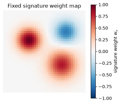

2. Simulate new test subjects’ condition images¶

Thirty new subjects, three conditions each:

pain — the target condition; expresses the signature strongly (amplitude ≈ 1.0, varying across subjects)
sound — an arousing but non-painful control; expresses the signature weakly (a confusable condition, in the spirit of Figure 40.2)
warmth — a neutral control; no signature expression

Each subject also gets a baseline (global) offset shared across their conditions, plus independent voxel noise — the kinds of nuisance variation real condition images carry.

rng = np.random.default_rng(2026)  # seed, for reproducibility
n_sub = 30                                # number of new test subjects

amp_pain  = rng.normal(1.0, 0.4, n_sub)   # target: strong expression
amp_sound = rng.normal(0.3, 0.2, n_sub)   # confusable control: weak expression
amp_warm  = np.zeros(n_sub)               # neutral control: none

offset   = rng.normal(0, 0.3, n_sub)      # subject baseline (global) differences
noise_sd = 4.0                            # voxel noise

def make_condition_images(amp):
    return (amp[:, None] * w + offset[:, None]
            + noise_sd * rng.standard_normal((n_sub, n_vox)))

img_pain  = make_condition_images(amp_pain)    # subjects x voxels
img_sound = make_condition_images(amp_sound)
img_warm  = make_condition_images(amp_warm)

fig, axes = plt.subplots(1, 2, figsize=(7, 3))
axes[0].imshow(W, cmap="RdBu_r", vmin=-1, vmax=1)
axes[0].set_title("Signature")
axes[1].imshow(img_pain[0].reshape(side, side), cmap="RdBu_r", vmin=-8, vmax=8)
axes[1].set_title("Subject 1, pain image (noisy)")
for ax in axes:
    ax.axis("off")
plt.tight_layout()
plt.show()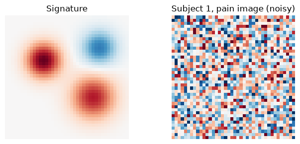

Notice that the signature is invisible to the eye in any single noisy image. The whole point of a multivariate pattern is that a weighted sum across thousands of voxels can recover a signal no single voxel shows reliably.

3. Pattern responses: the dot product¶

The pattern response for an image $\mathbf{x}$ is

r = \mathbf{w}^\top \mathbf{x} = \sum_{v=1}^{V} w_v\, x_v

(1)

r — pattern response (signature score) · w — fixed signature weights (voxels × 1) · x — brain image as a vector (voxels × 1) · wᵥ, xᵥ — weight and image value at voxel v · V — number of voxels

where $r$ is the pattern response (the signature’s score for the image), $\mathbf{w}$ the fixed vector of signature weights (one per voxel), $\mathbf{x}$ the brain image arranged as a vector, $w_v$ and $x_v$ their values at voxel $v$ , and $V$ the number of voxels.

a weighted average of image values with weights fixed by the signature. (With CANlab tools this is apply_mask(data_obj, signature, 'pattern_expression', 'ignore_missing'); with nilearn you would mask both images to a common space and take the dot product, exactly as below.)

resp = {"pain": img_pain @ w, "sound": img_sound @ w, "warmth": img_warm @ w}

plt.figure(figsize=(5.5, 3.8))
for s in range(n_sub):   # connect each subject's conditions
    plt.plot([0, 1, 2], [resp["pain"][s], resp["sound"][s], resp["warmth"][s]],
             "-", color="gray", alpha=0.25, lw=0.7)
for i, (name, r) in enumerate(resp.items()):
    plt.plot(np.full(n_sub, i) + rng.uniform(-.06, .06, n_sub), r, "o", alpha=.65,
             label=name)
plt.xticks([0, 1, 2], list(resp))
plt.ylabel(r"Pattern response  $w^\top x$")
plt.title("Signature responses by condition (lines = subjects)")
plt.tight_layout()
plt.show()

print("Mean responses:", {k: round(float(v.mean()), 1) for k, v in resp.items()})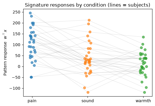

Mean responses: {'pain': 104.8, 'sound': 37.4, 'warmth': 12.8}

The response is graded — largest for pain, intermediate for the arousing sound, near zero for warmth — mirroring how a well-designed signature should track its target construct across a dynamic range rather than just separating two arbitrary classes.

4. Paired forced-choice accuracy¶

The natural within-person test: for each subject, which condition produced the larger pattern response? Because both responses come from the same person, baseline (offset) differences between subjects cancel. We test accuracy against chance (50%) with a binomial test.

def forced_choice(a, b):
    k = int(np.sum(a > b))
    acc = k / n_sub
    p = stats.binomtest(k, n_sub, 0.5).pvalue
    return acc, p

for c1, c2 in [("pain", "warmth"), ("pain", "sound"), ("sound", "warmth")]:
    acc, p = forced_choice(resp[c1], resp[c2])
    print(f"{c1:>6} vs {c2:<7}  forced-choice accuracy = {acc:.2f}  (binomial p = {p:.2g})")

  pain vs warmth   forced-choice accuracy = 0.97  (binomial p = 5.8e-08)
  pain vs sound    forced-choice accuracy = 0.77  (binomial p = 0.0052)
 sound vs warmth   forced-choice accuracy = 0.67  (binomial p = 0.099)

Pain vs. warmth discrimination is excellent; pain vs. the confusable sound condition is harder — that gap between the two comparisons is a measure of the signature’s specificity, and it is only visible because the test set includes a confusable control condition (sample design at work).

5. ROC curves, sensitivity, and specificity¶

For single-interval classification — deciding from one image alone, with one threshold applied to everyone — we trace the ROC curve, compute the area under it (AUC), and read off sensitivity and specificity at the best balanced threshold (Youden’s J).

plt.figure(figsize=(4.5, 4.2))
for ctrl, color in [("warmth", "tab:blue"), ("sound", "tab:orange")]:
    y = np.r_[np.ones(n_sub), np.zeros(n_sub)]
    v = np.r_[resp["pain"], resp[ctrl]]
    fpr, tpr, thr = roc_curve(y, v)
    auc = roc_auc_score(y, v)
    j = np.argmax(tpr - fpr)                 # Youden's J: best balanced threshold
    plt.plot(fpr, tpr, color=color, label=f"pain vs {ctrl}: AUC = {auc:.2f}")
    plt.plot(fpr[j], tpr[j], "o", color=color)
    print(f"pain vs {ctrl:<7}  AUC = {auc:.2f} | at best threshold: "
          f"sensitivity = {tpr[j]:.2f}, specificity = {1 - fpr[j]:.2f}")

plt.plot([0, 1], [0, 1], "k:", lw=1)
plt.xlabel("1 - specificity (false positive rate)")
plt.ylabel("sensitivity (true positive rate)")
plt.title("Single-interval ROC")
plt.legend(loc="lower right")
plt.tight_layout()
plt.show()

pain vs warmth   AUC = 0.84 | at best threshold: sensitivity = 0.73, specificity = 0.87
pain vs sound    AUC = 0.75 | at best threshold: sensitivity = 0.83, specificity = 0.67

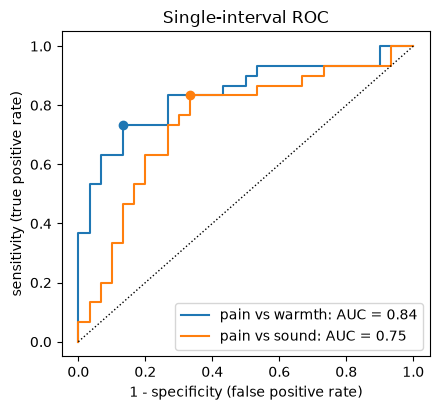
Compare the single-interval sensitivity/specificity with the forced-choice accuracies above: forced choice does better, because between-subject baseline variance — which a single threshold must fight through — cancels in the paired comparison. Published signatures (e.g., the Neurologic Pain Signature) show exactly this pattern: forced-choice accuracy is typically the highest-powered test.

6. Metric choice and calibration across scanners¶

The dot product is not the only way to compare an image with a pattern:

dot product $\mathbf{w}^\top\mathbf{x}$ — keeps the image’s units; sensitive to scanner gain and offset
cosine similarity $\mathbf{w}^\top\mathbf{x} / (\lVert\mathbf{w}\rVert \lVert\mathbf{x}\rVert)$ — invariant to multiplicative gain, still sensitive to additive offsets
correlation — cosine similarity after mean-centering both vectors; invariant to gain and uniform offset

Suppose the same subjects’ pain images had come from “Scanner B”, which scales signal by 1.8× and adds a uniform offset. Watch what happens to each metric.

def pattern_metrics(X, w):
    dot = X @ w
    cos = dot / (np.linalg.norm(X, axis=1) * np.linalg.norm(w))
    Xc = X - X.mean(axis=1, keepdims=True)
    wc = w - w.mean()
    corr = (Xc @ wc) / (np.linalg.norm(Xc, axis=1) * np.linalg.norm(wc))
    return {"dot product": dot, "cosine": cos, "correlation": corr}

gain, shift = 1.8, 5.0                        # Scanner B: multiplicative gain, additive offset
img_pain_B = gain * img_pain + shift          # same brains, different scanner

mA = pattern_metrics(img_pain, w)
mB = pattern_metrics(img_pain_B, w)

fig, axes = plt.subplots(1, 3, figsize=(9.5, 3.2))
for ax, name in zip(axes, mA):
    ax.boxplot([mA[name], mB[name]])
    ax.set_xticklabels(["Scanner A", "Scanner B"])
    ax.set_title(name)
fig.suptitle("Same brains, different scanner gain/offset")
plt.tight_layout()
plt.show()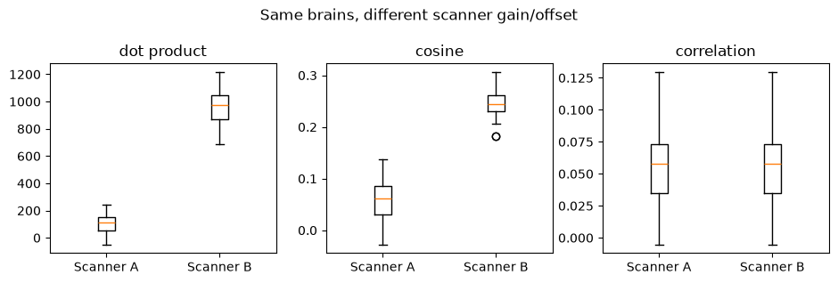

# Within-scanner, within-person comparisons survive the transformation:
img_warm_B = gain * img_warm + shift
acc_A = np.mean(resp["pain"] > resp["warmth"])
acc_B = np.mean(img_pain_B @ w > img_warm_B @ w)
print(f"Forced-choice accuracy (pain vs warmth), Scanner A: {acc_A:.2f}")
print(f"Forced-choice accuracy (pain vs warmth), Scanner B: {acc_B:.2f}")

Forced-choice accuracy (pain vs warmth), Scanner A: 0.97
Forced-choice accuracy (pain vs warmth), Scanner B: 0.97

The raw dot product shifts dramatically between scanners — pooling it across sites without harmonization would be misleading. Cosine similarity removes the gain but not the offset; correlation is robust to both. And the paired forced-choice accuracy is identical on both scanners, because within-person comparisons are invariant to any transformation applied equally to a subject’s conditions.

Summary¶

A population-level signature is a fixed weight map; its response to a new image is the dot product $\mathbf{w}^\top\mathbf{x}$ — a pattern-weighted generalization of the ROI average. It is never re-fit to test data.
Responses should be graded across conditions; testing against confusable controls (not just neutral ones) quantifies specificity.
Paired forced-choice tests are high-powered because subject baselines cancel; single-interval ROC/sensitivity/specificity characterize threshold-based classification.
Metric choice matters for calibration across scanners: dot products are scale- and offset-sensitive, cosine similarity is gain-invariant, correlation is gain- and offset-invariant — and within-person comparisons are the most robust of all.

Next, Chapter 41 takes up what it means for such a signature to become a validated neuromarker.