Chapter 41 Lab — Biomarkers and Translational Neuroscience (Python) - Elements of fMRI Analysis

In this lab you will build the quantitative toolkit for evaluating brain-based biomarkers: converters among effect size ( $d$ ), classification accuracy, AUC, and number needed to treat (NNT); a simulation of the winner’s curse showing why discovery effect sizes shrink on replication; and a diagnostic testing analysis showing how base rates govern the meaning of a positive test.

How to run this: This notebook runs in your browser (via Pyodide), on Colab, or locally — it uses only numpy, scipy, and matplotlib on simulated data, so no downloads are needed. Run cells top to bottom. It accompanies the chapter page 41. Biomarkers and Translational Neuroscience.

Code adapted from CANlab FMRI_simulations (github.com/canlab): effect_size_formulas.m, effect_size_vs_classification_accuracy.m, Cohens_d_to_NNT.mlx, effect_size_inflation_example_sim.m, and diagnostic_testing.m.

Part 1 — Effect size converters¶

Under a normal, equal-variance model — controls $\sim N(0, 1)$ , patients $\sim N(d, 1)$ — the key clinical performance metrics are exact functions of $d$ :

Point-biserial correlation: $r = d / \sqrt{d^2 + 4}$
Forced-choice accuracy (given one patient and one control, pick the patient) — which equals the area under the ROC curve: $\mathrm{AUC} = \Phi(d/\sqrt{2})$
Single-interval accuracy (classify one person against a fixed cutpoint): $\Phi(d/2)$
Number needed to treat (Furukawa): $\mathrm{NNT} = 1 / \left[\Phi\left(d + \Phi^{-1}(\mathrm{CER})\right) - \mathrm{CER}\right]$ , where CER is the control-group event rate

Forced choice is easier than single-interval classification (you get to compare two observations), so the same $d$ yields higher accuracy.

▶ This notebook is interactive. Click the ⏻ power icon at the top right of this page to run it in your browser — no installation needed (the kernel takes ~30–60 s to start the first time). Then run cells top to bottom, starting with the first code cell below: later cells depend on the imports and variables defined earlier, and will error if you skip ahead.

import numpy as np
import matplotlib.pyplot as plt
from scipy import stats
from scipy.stats import norm
import pandas as pd

# Effect size converters (normal, equal-variance model)
d2r        = lambda d: d / np.sqrt(d**2 + 4)            # d -> point-biserial r
r2d        = lambda r: 2 * r / np.sqrt(1 - r**2)        # r -> d
d2acc_forc = lambda d: norm.cdf(d / np.sqrt(2))         # forced-choice acc = AUC
d2acc_sing = lambda d: norm.cdf(d / 2)                  # single-interval accuracy
acc2d_sing = lambda a: 2 * norm.ppf(a)                  # accuracy -> required d
d2nnt      = lambda d, cer: 1 / (norm.cdf(d + norm.ppf(cer)) - cer)  # Furukawa
auc2nnt    = lambda auc: 1 / (2 * auc - 1)              # Kraemer & Kupfer

# Reference table: small / medium / large effects, plus the NPS response
# to evoked pain (d = 2.32 across 20 independent studies)
d_ref = np.array([0.2, 0.5, 0.8, 1.5, 2.32])
table = pd.DataFrame({
    "d": d_ref,
    "r": d2r(d_ref).round(2),
    "acc_single": (100 * d2acc_sing(d_ref)).round(1),
    "AUC": d2acc_forc(d_ref).round(3),
    "NNT (CER=0.5)": d2nnt(d_ref, 0.5).round(1),
})
print(table.to_string(index=False))
print(f"\nd required for 90% accuracy, single interval: {acc2d_sing(0.9):.2f}")
print(f"d required for 90% accuracy, forced choice:   {np.sqrt(2)*norm.ppf(0.9):.2f}")

   d    r  acc_single   AUC  NNT (CER=0.5)
0.20 0.10        54.0 0.556           12.6
0.50 0.24        59.9 0.638            5.2
0.80 0.37        65.5 0.714            3.5
1.50 0.60        77.3 0.856            2.3
2.32 0.76        87.7 0.950            2.0

d required for 90% accuracy, single interval: 2.56
d required for 90% accuracy, forced choice:   1.81

Note the punchline: a conventionally “large” effect of $d = 0.8$ classifies individuals at only ~66% — barely better than a coin flip. Confident individual-level decisions require effects in the $d \ge 2$ range, like the NPS response to evoked pain.

# Plot accuracy and AUC as a function of d
d = np.arange(0, 3.01, 0.02)       # effect sizes to plot, 0 to 3

fig, ax = plt.subplots(figsize=(7, 5))
ax.plot(d, d2acc_forc(d), lw=3, label="Forced choice (= AUC)")
ax.plot(d, d2acc_sing(d), lw=3, label="Single interval")
ax.axhline(0.5, ls=":", color="k", lw=2, label="Chance")

# Crosshairs: what does d = 0.8 buy you? What d do you need for 90%?
for d_mark, acc_fun in [(0.8, d2acc_sing), (acc2d_sing(0.9), d2acc_sing)]:
    a = acc_fun(d_mark)
    ax.plot([d_mark, d_mark], [0.5, a], "k--", lw=1)
    ax.plot([0, d_mark], [a, a], "k--", lw=1)
    ax.text(d_mark, 0.46, f"{d_mark:.1f}", ha="center", fontsize=12)

ax.set(xlabel="Effect size (d)", ylabel="Classification accuracy",
       ylim=(0.4, 1.02), title="Accuracy by effect size")
ax.legend(loc="lower right")
plt.tight_layout()
plt.show()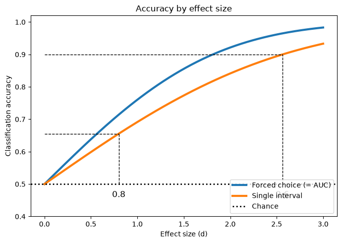

Part 2 — Verify the formulas by simulation¶

Formulas are only trustworthy if we can reproduce them from first principles. Simulate a large sample of controls and patients and measure both kinds of accuracy empirically.

rng = np.random.default_rng(1)     # seed for reproducibility
d_true, n = 0.8, 200_000           # d_true = group separation; n = draws per group

controls = rng.standard_normal(n)            # N(0, 1)
patients = d_true + rng.standard_normal(n)   # N(d, 1)

# Forced choice: pair one patient with one control, pick the higher score
emp_forced = np.mean(patients > controls)

# Single interval: classify one observation against the optimal cutpoint
# (midway between the means when variances are equal)
cut = d_true / 2
emp_single = np.mean(np.concatenate([patients > cut, controls <= cut]))

# AUC computed nonparametrically from the ROC (rank statistic)
emp_auc = stats.mannwhitneyu(patients, controls).statistic / n**2

print(f"Forced choice:   theory {d2acc_forc(d_true):.3f}, simulated {emp_forced:.3f}")
print(f"Single interval: theory {d2acc_sing(d_true):.3f}, simulated {emp_single:.3f}")
print(f"AUC:             theory {d2acc_forc(d_true):.3f}, simulated {emp_auc:.3f}")

Forced choice:   theory 0.714, simulated 0.714
Single interval: theory 0.655, simulated 0.656
AUC:             theory 0.714, simulated 0.715

# Visualize the two class distributions and the misclassification zones
x = np.linspace(-4, 5, 400)
f_ctrl, f_pat = norm.pdf(x), norm.pdf(x, loc=d_true)

fig, ax = plt.subplots(figsize=(7, 4))
ax.fill_between(x, f_ctrl, alpha=0.3, color="crimson", label="Controls")
ax.fill_between(x, f_pat, alpha=0.3, color="royalblue", label=f"Patients (d = {d_true})")
ax.axvline(cut, color="k", lw=2, label="Optimal cutpoint (d/2)")
ax.fill_between(x[x >= cut], f_ctrl[x >= cut], color="crimson", alpha=0.7)
ax.fill_between(x[x < cut], f_pat[x < cut], color="royalblue", alpha=0.7)
ax.set(xlabel="Biomarker response", ylabel="Probability density",
       title="Single-interval classification: dark areas are misclassified")
ax.legend()
plt.tight_layout()
plt.show()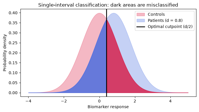

Part 3 — From $d$ to number needed to treat¶

NNT answers the clinician’s question: how many patients must I treat for one additional success relative to control? It is the reciprocal of the difference in event rates, $\mathrm{NNT} = 1/(\mathrm{EER} - \mathrm{CER})$ .

Converting a continuous effect $d$ to NNT requires defining a “response” threshold on the outcome scale, summarized by the control event rate (CER). We verify Furukawa’s formula by direct simulation, and compare the threshold-free Kraemer & Kupfer variant, $\mathrm{NNT} = 1/(2\,\mathrm{AUC} - 1)$ .

d_true = 0.5                       # treatment effect size
thr = 0.0                          # response = outcome above this threshold
cer = 1 - norm.cdf(thr)            # control event rate = 0.5 here

x_ctrl  = rng.standard_normal(n)
x_treat = d_true + rng.standard_normal(n)
eer_emp, cer_emp = np.mean(x_treat > thr), np.mean(x_ctrl > thr)
nnt_emp = 1 / (eer_emp - cer_emp)

print(f"NNT at d = {d_true}, CER = {cer:.2f}:")
print(f"  Furukawa formula:  {d2nnt(d_true, cer):.1f}")
print(f"  Direct simulation: {nnt_emp:.1f}")
print(f"  Kraemer & Kupfer (threshold-free): {auc2nnt(d2acc_forc(d_true)):.1f}")

NNT at d = 0.5, CER = 0.50:
  Furukawa formula:  5.2
  Direct simulation: 5.2
  Kraemer & Kupfer (threshold-free): 3.6

# NNT depends strongly on the response criterion
cer_vals = np.arange(0.02, 0.91, 0.01)   # response criteria, stringent to lenient

fig, ax = plt.subplots(figsize=(7, 5))
for d_val in [0.2, 0.5, 0.8, 1.2]:       # effect sizes to compare
    ax.plot(cer_vals, d2nnt(d_val, cer_vals), lw=3, label=f"d = {d_val}")
ax.set_yscale("log")
ax.set(xlabel="Control event rate (CER)", ylabel="NNT (log scale)",
       title="NNT as a function of d and response criterion")
ax.legend()
plt.tight_layout()
plt.show()

print("With d = 0.5, NNT ranges from "
      f"{d2nnt(0.5, 0.5):.0f} (lenient criterion, CER = 0.5) to "
      f"{d2nnt(0.5, 0.02):.0f} (stringent criterion, CER = 0.02).")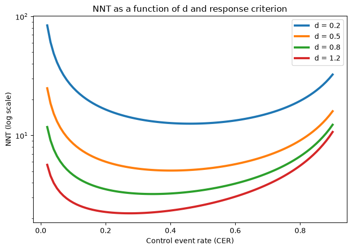

With d = 0.5, NNT ranges from 5 (lenient criterion, CER = 0.5) to 25 (stringent criterion, CER = 0.02).

The same drug, the same $d$ — but the NNT can differ by an order of magnitude depending on how “response” is defined. Clinical claims are meaningless without the criterion attached.

Part 4 — The winner’s curse: inflated discovery effect sizes¶

When many tests are performed (voxels, regions, candidate models) and results are selected for significance or top performance, the selected effect sizes are biased upward — a significant result in a small sample must have a large observed effect, and chance supplied part of it. We simulate a discovery study with 5,000 voxels that all carry the same true effect, select the significant ones, then re-measure exactly those voxels in an independent replication study.

rng = np.random.default_rng(42)    # seed for reproducibility
n_vox, n_sub, d_true = 5000, 20, 0.5   # tests (voxels), subjects, true effect everywhere
alpha_v = 0.001                    # voxelwise significance threshold

# Discovery study: one-sample t-test at each voxel (subjects x voxels)
Y_disc = d_true + rng.standard_normal((n_sub, n_vox))
t_disc, p_disc = stats.ttest_1samp(Y_disc, 0)
d_disc = Y_disc.mean(axis=0) / Y_disc.std(axis=0, ddof=1)   # observed d

sig = (p_disc < alpha_v) & (d_disc > 0)
print(f"{sig.sum()} of {n_vox} voxels significant at p < {alpha_v}")

# Replication study: same voxels, new subjects, NO selection
Y_rep = d_true + rng.standard_normal((n_sub, n_vox))
d_rep = Y_rep.mean(axis=0) / Y_rep.std(axis=0, ddof=1)

print(f"True d everywhere:                              {d_true:.2f}")
print(f"Mean observed d, significant voxels (discovery): {d_disc[sig].mean():.2f}")
print(f"Mean observed d, same voxels (replication):      {d_rep[sig].mean():.2f}")

408 of 5000 voxels significant at p < 0.001
True d everywhere:                              0.50
Mean observed d, significant voxels (discovery): 1.02
Mean observed d, same voxels (replication):      0.54

fig, ax = plt.subplots(figsize=(7, 5))
bins = np.linspace(-0.5, 2.0, 40)
ax.hist(d_disc[sig], bins=bins, alpha=0.55, color="crimson",
        label="Discovery (selected voxels)")
ax.hist(d_rep[sig], bins=bins, alpha=0.55, color="royalblue",
        label="Replication (same voxels)")
ax.axvline(d_true, color="k", ls="--", lw=2, label=f"True d = {d_true}")
ax.set(xlabel="Observed effect size (d)", ylabel="Number of voxels",
       title="Winner's curse: selected effects shrink on replication")
ax.legend()
plt.tight_layout()
plt.show()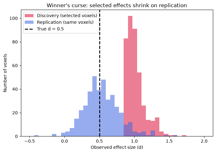

The significant voxels looked like $d \approx 1$ in the discovery sample — double the truth. In the replication sample, the same voxels return to an unbiased $d \approx 0.5$ . Nothing about the brain changed; only the selection did. The same mechanism inflates cross-validated accuracy when analysts try several models and report the best one.

How bad can it get? Even with no true effect anywhere, selecting the maximum across many tests manufactures large apparent effects — worse for small samples:

# Expected max-|Z| across v null tests, converted to d for several sample sizes
# (adapted from expected_effect_size_inflation_curve.m)
rng = np.random.default_rng(7)     # seed for reproducibility
n_tests = np.unique(np.round(np.logspace(0, 5, 30)).astype(int))  # number of tests: 1 to 100,000
n_vals = [10, 20, 30, 100]         # sample sizes to compare
nsim = 2000                        # simulations per point; more gives smoother curves

d_inflate = np.zeros((len(n_tests), len(n_vals)))
for v, nt in enumerate(n_tests):
    # expected maximum Z across nt independent null tests
    z_max = rng.standard_normal((nsim, nt)).max(axis=1).mean()
    p_max = 1 - norm.cdf(z_max)
    for i, n_s in enumerate(n_vals):
        t_equiv = stats.t.ppf(1 - p_max, df=n_s - 1)
        d_inflate[v, i] = t_equiv / np.sqrt(n_s)

fig, ax = plt.subplots(figsize=(7, 5))
for i, n_s in enumerate(n_vals):
    ax.plot(np.log(n_tests), d_inflate[:, i], lw=3, label=f"n = {n_s}")
ax.axhline(0, ls="--", color="gray")
ax.set(xlabel="Log number of tests performed",
       ylabel="Expected max observed d under the null",
       title="Effect size inflation from selection alone (true d = 0)")
ax.legend()
plt.tight_layout()
plt.show()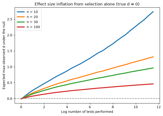

With $n = 20$ and hundreds of thousands of voxel tests, the expected maximum effect under the pure null already exceeds $d = 1$ — “whopping” effects can be produced by selection alone. This is why unbiased effect sizes and performance estimates require prospective tests on independent data with all model parameters frozen.

Part 5 — Diagnostic testing: base rates and PPV¶

Sensitivity and specificity are properties of the test. But the question a patient cares about — given a positive result, do I have the condition? — is the positive predictive value, and it depends on the prevalence (base rate) in the tested population:

\mathrm{PPV} = \frac{\mathrm{sens} \cdot \mathrm{prev}}{\mathrm{sens} \cdot \mathrm{prev} + (1 - \mathrm{spec})(1 - \mathrm{prev})}

(1)

PPV — probability that a positive test is a true positive · sens — sensitivity: P(test + | condition present) · spec — specificity: P(test − | condition absent) · prev — prevalence (base rate) in the tested population

where $\mathrm{PPV}$ is the probability that a positive test is a true positive, $\mathrm{sens}$ the sensitivity, $\mathrm{spec}$ the specificity, and $\mathrm{prev}$ the prevalence of the condition in the tested population.

def calc_ppv(sens, spec, prev):
    return sens * prev / (sens * prev + (1 - spec) * (1 - prev))

def calc_npv(sens, spec, prev):
    return spec * (1 - prev) / ((1 - sens) * prev + spec * (1 - prev))

# An excellent test meets a rare condition
for sens, spec, prev in [(.98, .98, .10), (.98, .98, .01), (.98, .98, .001),
                         (.98, .999, .001)]:
    print(f"sens {sens:.0%}, spec {spec:.1%}, prevalence {prev:.1%}: "
          f"PPV = {calc_ppv(sens, spec, prev):.2f}")

sens 98%, spec 98.0%, prevalence 10.0%: PPV = 0.84
sens 98%, spec 98.0%, prevalence 1.0%: PPV = 0.33
sens 98%, spec 98.0%, prevalence 0.1%: PPV = 0.05
sens 98%, spec 99.9%, prevalence 0.1%: PPV = 0.50

Even at 98% sensitivity and specificity, a positive test for a condition affecting 1% of people is correct only one time in three — and for a 1-in-1000 condition, specificity must approach 99.9% before PPV is even a coin flip. This is why screening for rare disorders is so hard, and why a brain biomarker’s specificity must be established against many alternative conditions, not just healthy controls.

# PPV as a function of prevalence and test properties
prev = np.linspace(0.005, 0.5, 200)      # prevalence (base rate) range to sweep
fig, axes = plt.subplots(1, 2, figsize=(11, 4.5), sharey=True)

for spec in [0.80, 0.90, 0.95, 0.98, 0.999]:
    axes[0].plot(prev, calc_ppv(0.90, spec, prev), lw=3, label=f"spec = {spec:.3f}")
axes[0].set(xlabel="Prevalence", ylabel="Positive predictive value",
            title="Sensitivity fixed at 90%")
axes[0].legend(fontsize=9)

for sens in [0.60, 0.75, 0.90, 0.99]:
    axes[1].plot(prev, calc_ppv(sens, 0.90, prev), lw=3, label=f"sens = {sens:.2f}")
axes[1].set(xlabel="Prevalence", title="Specificity fixed at 90%")
axes[1].legend(fontsize=9)

plt.tight_layout()
plt.show()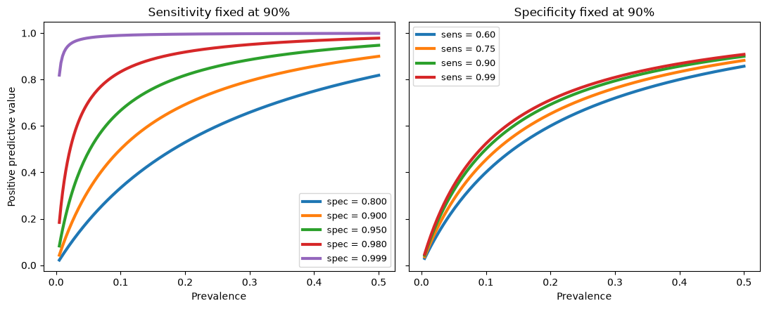

Compare the two panels: varying specificity fans the curves apart dramatically, while varying sensitivity barely moves them. PPV is driven by specificity and prevalence; sensitivity matters mainly for the negative predictive value.

A realistic scenario. Current brain biomarkers for chronic pain classify patients vs. healthy controls at roughly 90% sensitivity / 80% specificity. Suppose one is deployed in a clinic where 20% of tested patients truly have the target condition:

sens, spec, prev = 0.90, 0.80, 0.20    # test properties; prev = clinic base rate
print(f"Realistic biomarker (sens {sens:.0%}, spec {spec:.0%}, prev {prev:.0%}):")
print(f"  PPV = {calc_ppv(sens, spec, prev):.2f}   "
      f"(a positive test is right about half the time)")
print(f"  NPV = {calc_npv(sens, spec, prev):.2f}   "
      f"(a negative test is quite reassuring)")
print()
print("Where should development effort go?")
print(f"  Improve specificity to 95%: PPV -> {calc_ppv(0.90, 0.95, prev):.2f}")
print(f"  Improve sensitivity to 99%: PPV -> {calc_ppv(0.99, 0.80, prev):.2f}")

# Expected performance per 1000 patients tested
n_pop = 1000                           # hypothetical number of patients tested
tp = sens * prev * n_pop; fp = (1 - spec) * (1 - prev) * n_pop
fn = (1 - sens) * prev * n_pop; tn = spec * (1 - prev) * n_pop
print(f"\nPer 1000 patients: {tp:.0f} true pos, {fp:.0f} FALSE pos, "
      f"{tn:.0f} true neg, {fn:.0f} false neg")

Realistic biomarker (sens 90%, spec 80%, prev 20%):
  PPV = 0.53   (a positive test is right about half the time)
  NPV = 0.97   (a negative test is quite reassuring)

Where should development effort go?
  Improve specificity to 95%: PPV -> 0.82
  Improve sensitivity to 99%: PPV -> 0.55

Per 1000 patients: 180 true pos, 160 FALSE pos, 640 true neg, 20 false neg

Wrap-up¶

Effect sizes translate into clinical metrics — $r$ , accuracy, AUC, and NNT are interconvertible under normal assumptions. Report the ones that answer the clinical question, with criteria attached.
A “large” effect is not a biomarker. $d = 0.8$ classifies individuals at ~66%; useful individual-level decisions need $d \gtrsim 2$ , achievable so far mainly for states like evoked pain rather than trait diagnoses.
Selection inflates. Effects chosen for significance or top performance shrink on replication; only prospective tests of frozen models on independent data give unbiased estimates.
Base rates rule deployment. PPV depends on prevalence and specificity; a biomarker validated against healthy controls at 80% specificity yields only ~50% PPV in realistic clinical use — specificity against other conditions is the frontier.

These are the quantitative teeth behind the chapter’s five criteria for useful brain signatures: precise definition, person-level diagnosticity, interpretability, deployability, and generalizability.

Chapter 41 Lab — Biomarkers and Translational Neuroscience (Python)