35. Dynamic Causal Models - Elements of fMRI Analysis

Dynamic Causal Models¶

What you will learn

Why dynamic causal modeling (DCM) moves effective connectivity analysis from the observed BOLD level to the latent neuronal level, using a generative state-space model
How the bilinear neuronal model $\dot{z} = (A + \sum_j u_j B^{(j)})z + Cu$ separates intrinsic coupling ( $A$ ), input-induced changes in coupling ( $B$ ), and direct driving inputs ( $C$ )
How an extended Balloon model maps neuronal states to predicted BOLD signals, and why hemodynamic parameters are estimated with shrinkage priors
How Bayesian model inversion yields posterior distributions over connection strengths, and how model evidence and Bayes factors support comparing candidate network models
The key caveats — model misspecification, omitted regions, and small networks — and current extensions (regression, stochastic, and spectral DCM)

Run this code: ⚡ In-browser lab · Colab · MATLAB Online

Overview¶

Most effective connectivity methods, including the structural equation and path models of Chapter 34, operate directly on the observed BOLD time series. But BOLD observations are several layers removed from the neuronal activity we actually care about, which limits how far results can be interpreted at the neuronal level. Dynamic causal modeling takes a different approach: it treats the observed data as outputs of latent (unobserved) neuronal activity. A DCM for fMRI combines a neurodynamic model of interacting brain regions with a hemodynamic model describing how neuronal activity is transformed into blood flow and, ultimately, the measured BOLD signal. Together these form a generative (forward) model: given neuronal signals and parameters, it predicts what data we should observe.

DCM is built on a state-space design that treats the brain as a deterministic, nonlinear dynamic system receiving inputs and producing outputs. The first equation describes how experimental manipulations influence the dynamics of the latent neuronal states $z$ :

\dot{z} = f(z, u, \theta)

(1)

ż — rate of change of the latent neuronal states · z — neuronal states of the modeled regions · u — exogenous (task) inputs · θ — path coefficients (connectivity parameters) · f — function describing the neuronal dynamics

where $\dot{z}$ is the rate of change of the latent neuronal states $z$ , $u$ holds the exogenous (task) inputs, $\theta$ contains the path coefficients — analogous to regression slopes — that capture connectivity strength, and $f$ describes the neuronal dynamics.

The second equation maps latent states to observed data:

y = g(z, \theta_h)

(2)

y — observed data (BOLD time series) · z — latent neuronal states · g — observation (hemodynamic) model · θₕ — hemodynamic parameters

where $y$ is the observed data, $g$ is — for fMRI — a hemodynamic model, and $\theta_h$ its parameters describing the biophysics that turn neural activity into a BOLD response.

In practice the latent signals and parameters are unknown, so the model must be inverted: Bayesian methods recover the most likely parameters given the observed data, and effective connectivity is parameterized as the coupling among latent neuronal variables. The central idea is that experimental inputs cause changes in effective connectivity at the neuronal level, which in turn cause changes in the observed data.

For fMRI, the neuronal level uses a bilinear approximation. Writing $z_t$ for the vector of neuronal states across the $K$ modeled regions at time $t$ , a bilinear Taylor approximation of $f$ gives:

\dot{z} = \Big(A + \sum_{j=1}^{J} u_j B^{(j)}\Big) z + C u

(3)

z — neuronal states (K regions) · u — J experimental inputs, uⱼ the j-th · A — intrinsic (endogenous) coupling (K × K) · B⁽ʲ⁾ — change in coupling induced by input j (K × K) · C — direct driving influence of inputs (K × J)

where $z$ holds the neuronal states of the $K$ regions, $u$ the $J$ inputs ( $u_j$ the $j$ -th), $A$ the intrinsic coupling among regions, $B^{(j)}$ the change in coupling induced by input $j$ , and $C$ the direct driving influence of inputs on regions.

The three coefficient matrices have distinct roles. $A$ ( $K \times K$ ) is the intrinsic connectivity: directional coupling among regions in the absence of input — it can be asymmetric, with unidirectional or bidirectional connections. Each $B^{(j)}$ ( $K \times K$ ) captures the change in coupling induced by input $j$ : how a task or context modulates intrinsic connections. $C$ ( $K \times J$ ) holds the extrinsic influences: how inputs directly drive activity levels in regions. As in SEM, the analyst specifies a reduced set of connections on theoretical grounds rather than allowing everything to influence everything, and model comparison adjudicates among candidate structures.

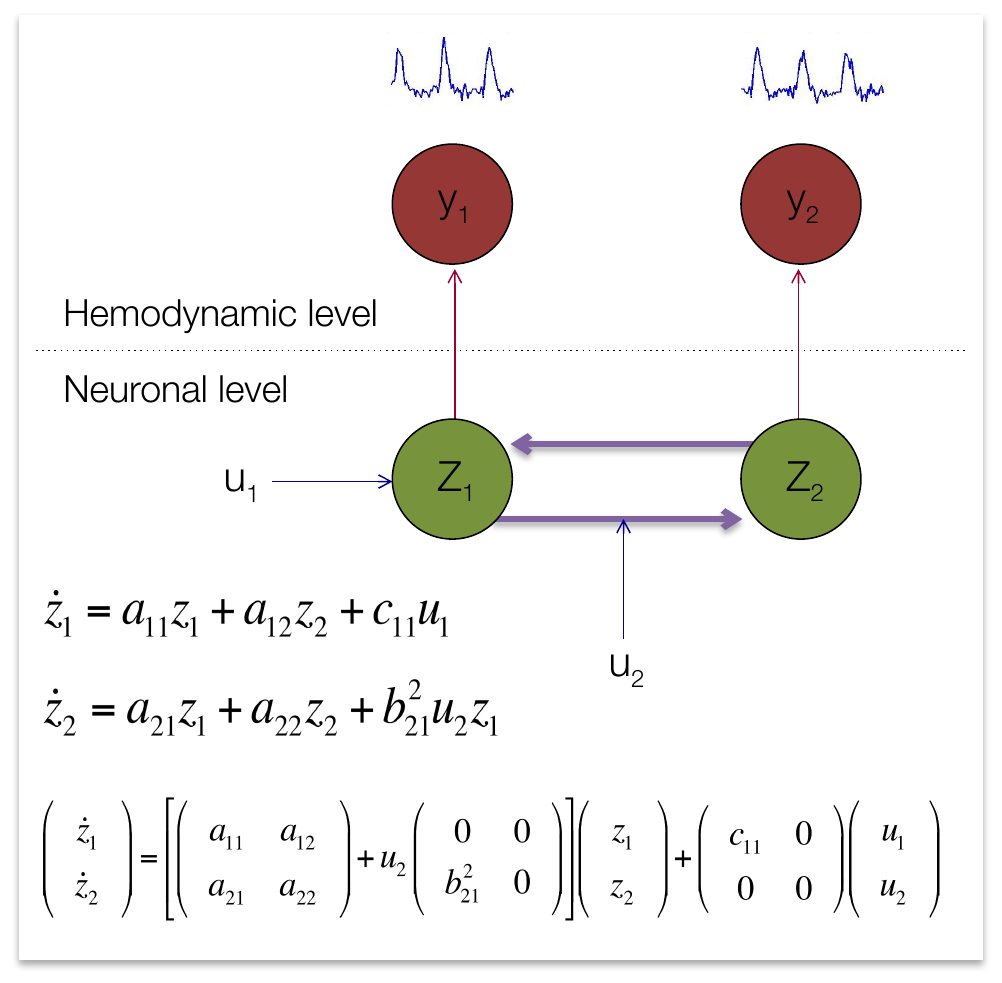
A two-region DCM with driving input u1 to region z1, modulatory input u2 acting on the z1-to-z2 connection, and hemodynamic transformation to observed signals y1 and y2, shown alongside the bilinear equations in scalar and matrix form — A simple DCM with two experimental inputs and two outputs. Input $u_1$ drives the level of neuronal state $z_1$ (via $c_{11}$ ), while $u_2$ modulates the $z_1 \to z_2$ connection (via $b^{2}_{21}$ ). Intrinsic coupling terms $a_{kl}$ make up the matrix $A$ . The latent neuronal states pass through a hemodynamic model to produce the predicted fMRI signals $y_1$ and $y_2$ . *(Figure 35.1 from the book. © the authors and MIT Press; reproduced with permission — not covered by this site’s CC-BY license.)*

The hemodynamic level is an extended Balloon model. Each region has four hemodynamic state variables — a vasodilatory signal, blood inflow, blood volume, and deoxyhemoglobin content — linked by differential equations, plus a fifth state for neuronal activity. Changes in neuronal activity generate a vasodilatory signal, increasing flow, volume, and changes in deoxygenation; as vessels “balloon” out they become less responsive to new input, creating a negative autoregulatory feedback loop. The predicted BOLD response is a nonlinear function of volume and deoxyhemoglobin content. For a brief stimulus the result resembles the canonical HRF, but the Balloon model is substantially more flexible and describes the process that produces that shape. Five hemodynamic parameters per region are estimated from the data, with Bayesian priors shrinking them toward canonical values.

Estimation inverts the combined neuronal-plus-hemodynamic state-space model with Bayesian methods: empirical priors on hemodynamic parameters, shrinkage priors on neural coupling parameters, and an Expectation–Maximization scheme that maximizes the posterior probability. The posterior over parameters is assumed Gaussian, and within-participant inference tests the probability that a connection exceeds a chosen threshold. To choose among candidate network structures, Bayesian model selection uses the model evidence — the marginal likelihood of the data under model $m$ :

p(y \mid m) = \int p(y \mid \theta, m)\, p(\theta \mid m)\, d\theta

(4)

p(y | m) — model evidence (marginal likelihood) · y — data concatenated across regions · m — candidate model · θ — model parameters, integrated out under their prior p(θ | m)

where $p(y \mid m)$ is the evidence for model $m$ , $y$ the time series concatenated across regions, and $\theta$ the model parameters, integrated out under their prior $p(\theta \mid m)$ .

and the Bayes factor comparing models $i$ and $j$ :

BF_{ij} = \frac{p(y \mid m_i)}{p(y \mid m_j)}

(5)

BF_ij — Bayes factor comparing models i and j · p(y | mᵢ), p(y | mⱼ) — model evidence for each candidate model

where $BF_{ij}$ is the Bayes factor and $p(y \mid m_i)$ , $p(y \mid m_j)$ are the evidences for candidate models $m_i$ and $m_j$ .

A large $BF_{ij}$ means the data favor model $i$ . One important restriction: only models containing the same set of regions (with different connections) can be compared this way — model selection cannot tell you whether to include a region in the first place. For group studies, the current standard is Parametric Empirical Bayes (PEB): all participants are assumed to share the same forward model but differ in connection strengths, and a second-level GLM on the participant-specific connection estimates (weighted by their posterior uncertainty) tests whether parameters are non-zero or differ between groups. When different, potentially non-nested models are fit per participant, models can instead be compared by cross-validated predictive accuracy in held-out data.

DCM is powerful and accessible — it unifies intrinsic effective connectivity with task-evoked activity and connectivity in a single model, and implementations are built into SPM with a graphical interface. But conclusions about direct influences and causality are only as good as the specified model. Omitting regions that influence the modeled ones can produce false inferences about the direction and strength of connections, and computational demands have traditionally limited DCMs to small networks (up to roughly 10 regions). As with mediation and other path models, the safest course is to use DCM to identify systems and pathways without making strong causal claims. Ongoing extensions address these limits: regression DCM reformulates the model as a Bayesian linear regression in the frequency domain, opening the door to whole-brain effective connectivity; stochastic and spectral DCM suit resting-state data; and hierarchical models support group studies.

Hands-on tutorial¶

DCM software performs full Bayesian inversion of the neuronal-plus-hemodynamic model (in SPM), but the logic fits in a few dozen lines. In this tutorial you will build the generative model yourself: simulate a two-region bilinear system in which a modulatory input strengthens the $z_1 \to z_2$ connection, pass the latent neuronal states through a hemodynamic (HRF) observation model, and then compare a “modulation” model against a “no-modulation” model with BIC as a simple stand-in for model evidence. No SPM or DCM toolbox is needed.

Step 1 — Simulate the latent neuronal dynamics. We integrate $\dot{z} = (A + u_2 B^{(2)})z + Cu_1$ with the Euler method: input $u_1$ delivers brief driving pulses to region 1, and input $u_2$ (a block “context”, like attention) modulates the $z_1 \to z_2$ connection.

MATLAB

Python

dt = 0.1;  T = 300;       % dt = integration step (s); T = total simulation time (s)
t = (0:dt:T-dt)';         % fine time grid
n = numel(t);             % number of integration steps

u1 = double(mod(t, 20) < 1);            % 1-s driving pulse every 20 s
u2 = double(mod(floor(t/60), 2) == 1);  % alternating 60-s modulatory blocks

A  = [-0.4  0; 0.3 -0.4];               % intrinsic coupling (z1 -> z2 = 0.3)
B2 = [0 0; 0.5 0];                      % u2 modulates the z1 -> z2 path
C  = [1; 0];                            % u1 drives region 1 only

z = zeros(n, 2);
for i = 1:n-1                           % Euler integration of dz/dt
    dz = (A + u2(i) * B2) * z(i, :)' + C * u1(i);
    z(i+1, :) = z(i, :) + dt * dz';
end
plot(t, z);  legend('z_1', 'z_2');  xlabel('Time (s)');

import numpy as np
import matplotlib.pyplot as plt

dt, T = 0.1, 300.0        # dt = integration step (s); T = total simulation time (s)
t = np.arange(0, T, dt)   # fine time grid
n = t.size                # number of integration steps

u1 = ((t % 20) < 1).astype(float)          # 1-s driving pulse every 20 s
u2 = ((t // 60) % 2 == 1).astype(float)    # alternating 60-s modulatory blocks

A  = np.array([[-0.4, 0.0], [0.3, -0.4]])  # intrinsic coupling (z1 -> z2 = 0.3)
B2 = np.array([[0.0, 0.0], [0.5, 0.0]])    # u2 modulates the z1 -> z2 path
C  = np.array([1.0, 0.0])                  # u1 drives region 1 only

z = np.zeros((n, 2))
for i in range(n - 1):                     # Euler integration of dz/dt
    dz = (A + u2[i] * B2) @ z[i] + C * u1[i]
    z[i + 1] = z[i] + dt * dz

plt.plot(t, z); plt.legend(["$z_1$", "$z_2$"]); plt.xlabel("Time (s)")

Example output: the latent neuronal states, with modulation-ON blocks shaded. Region 2’s responses are visibly larger during the modulation blocks — the same driving pulses arrive, but the effective coupling is $a_{21} + b_{21} = 0.8$ instead of 0.3:

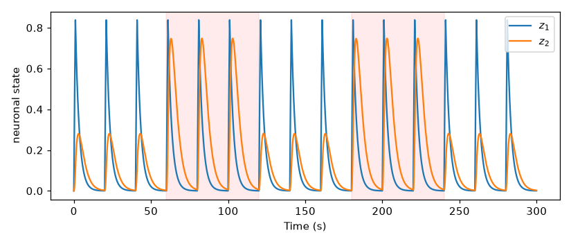
Time courses of the two latent neuronal states; region 1 responds identically to every pulse while region 2's responses roughly triple during the shaded modulatory blocks — Latent neuronal states $z_1$ and $z_2$ over the 300-s simulation (shaded intervals = modulatory input $u_2$ ON). Region 1 responds identically to every pulse; region 2’s responses grow whenever $u_2$ gates the $z_1 \to z_2$ connection.

Step 2 — Invert the model and compare hypotheses. After convolving the neuronal states with an HRF and sampling at the TR (the full labs build this observation model), we fit two candidate models to the noisy BOLD signal from region 2 — one with a free modulatory parameter $b_{21}$ , one with $b_{21} = 0$ — and score each with BIC, a simple proxy for log model evidence.

MATLAB

Python

% Fit each candidate by least squares (fit_dcm is defined in the full lab),
% then score with BIC = n*log(RSS/n) + k*log(n)
[rss1, k1] = fit_dcm(y2, true);    % modulation model: a21 and b21 free
[rss0, k0] = fit_dcm(y2, false);   % no-modulation model: b21 fixed at 0

n_obs = numel(y2);                 % number of BOLD samples (one per TR)
bic1 = n_obs * log(rss1 / n_obs) + k1 * log(n_obs);   % k1 = 2 free parameters
bic0 = n_obs * log(rss0 / n_obs) + k0 * log(n_obs);   % k0 = 1 free parameter
fprintf('dBIC (no-mod - mod) = %.1f -> evidence for modulation\n', bic0 - bic1)

# Fit each candidate by least squares (fit_dcm is defined in the full lab),
# then score with BIC = n*log(RSS/n) + k*log(n)
rss1, k1 = fit_dcm(y2, modulation=True)    # modulation model: a21, b21 free
rss0, k0 = fit_dcm(y2, modulation=False)   # no-modulation model: b21 = 0

n_obs = y2.size                    # number of BOLD samples (one per TR)
bic1 = n_obs * np.log(rss1 / n_obs) + k1 * np.log(n_obs)   # k1 = 2 free parameters
bic0 = n_obs * np.log(rss0 / n_obs) + k0 * np.log(n_obs)   # k0 = 1 free parameter
print(f"dBIC (no-mod - mod) = {bic0 - bic1:.1f} -> evidence for modulation")

Example output: the modulation model recovers the true coupling values and wins decisively:

Modulation model:    a21 = 0.314, b21 = 0.490 (truth: 0.300, 0.500)
No-modulation model: a21 = 0.509
BIC (modulation)    = -893.4
BIC (no modulation) = -688.4
dBIC (no-mod - mod) = 205.0 -> evidence for modulation

A large positive $\Delta$ BIC means the data strongly favor the modulation model — the same verdict a Bayes factor would deliver in a real DCM analysis, where BIC is replaced by a proper (free-energy) approximation to the log evidence. The full labs complete the arc: building the HRF observation model, visualizing observed versus fitted BOLD under both hypotheses, and re-running the comparison on data generated without modulation to confirm the evidence then favors the simpler model.

Go deeper

Open the full Python lab notebook → or download the MATLAB live script, which mirrors it.

Thought questions¶

SEM (Chapter 34) models covariances among observed BOLD signals, whereas DCM models coupling among latent neuronal states. What, concretely, does moving to the neuronal level buy you — and what new assumptions (neurodynamic and hemodynamic) are you paying with? When might the simpler observed-level model be the wiser choice?
Suppose an unmodeled region drives both regions in your two-region DCM with different conduction delays. Trace through how this omission could distort the estimated $A$ and $B$ matrices, and why a decisive Bayes factor between your candidate models would offer no protection against this error.
Bayesian model selection in DCM can only compare models containing the same set of regions. Explain why this restriction follows from the definition of model evidence, and formulate one scientific question about a three-region circuit that model selection can answer and one that it cannot.
In an attention study, attention could act by directly driving a motion-sensitive region (a $C$ effect) or by gating the connection from early visual cortex into it (a $B$ effect). What experimental design features and what patterns in the data would let a DCM distinguish these two accounts?
Hemodynamic parameters are estimated per region but shrunk toward canonical values by priors. Connect this to the flexibility–power tradeoff from Chapter 18: what could go wrong with fully free hemodynamics, what could go wrong with fully fixed ones, and how might regional hemodynamic differences masquerade as connectivity differences?

Quiz yourself¶

Cover of Elements of Functional Magnetic Resonance Imaging The book: Elements of Functional Magnetic Resonance Imaging — Wager & Lindquist, MIT Press

⌂ Back to home · Table of contents · How to use this site