Chapter 34 Lab — Structural Equation and Path Models (Python) - Elements of fMRI Analysis

In this lab you will build the core mediation-analysis workflow from scratch and fit a small path model — the observable-variable heart of structural equation modeling. The arc:

Simulate a brain-as-mediator dataset ( $X \to M \to Y$ plus a direct path)
Estimate the paths $a$ , $b$ , $c'$ , and $c$ with two regressions, and verify the decomposition $c = c' + ab$
Bootstrap a confidence interval and P value for the indirect effect $a \times b$
Break the model: show how an unmodeled confounder of the $M$ – $Y$ relationship manufactures a spurious indirect effect — and how adjusting for it repairs the analysis
Fit a three-node path model (the recursive SEM of Figure 34.1) by regression equations, compare the model-implied covariance with the observed one, and test an individual edge

How to run this notebook. It runs anywhere — directly in your browser on the tutorial site, on Colab, or locally — using only numpy, pandas, scipy, and matplotlib (no downloads, all data simulated). Run cells top to bottom. For the concepts behind the code, see the chapter page.

▶ This notebook is interactive. Click the ⏻ power icon at the top right of this page to run it in your browser — no installation needed (the kernel takes ~30–60 s to start the first time). Then run cells top to bottom, starting with the first code cell below: later cells depend on the imports and variables defined earlier, and will error if you skip ahead.

import numpy as np
import pandas as pd
import matplotlib.pyplot as plt
from scipy import stats

rng = np.random.default_rng(42)   # fix the random seed for reproducibility
np.set_printoptions(precision=3, suppress=True)
print("numpy", np.__version__, "| pandas", pd.__version__)

numpy 2.4.6 | pandas 3.0.5

Step 1 — Simulate a brain-as-mediator dataset¶

We mimic the chapter’s running example: a stressor manipulation $X$ , brain activity in an ACC region as the mediator $M$ , and stressor-evoked heart-rate increase as the outcome $Y$ . One observation per participant (single-level mediation), $n = 200$ .

The generative model is the mediation model, so we know the ground truth:

M_i = a\,X_i + e_{M,i}, \qquad Y_i = c'\,X_i + b\,M_i + e_{Y,i}

(1)

with true paths $a = 0.6$ , $b = 0.5$ , and direct effect $c' = 0.2$ . The implied total effect is $c = c' + ab = 0.2 + 0.30 = 0.50$ .

n = 200                                   # n = participants (one observation each)
a_true, b_true, cp_true = 0.6, 0.5, 0.2   # true paths: a (X->M), b (M->Y|X), c' (direct)

X = rng.standard_normal(n)                        # exposure (e.g., stressor intensity)
M = a_true * X + rng.standard_normal(n)           # mediator (e.g., ACC activity)
Y = cp_true * X + b_true * M + rng.standard_normal(n)  # outcome (e.g., heart rate)

fig, axes = plt.subplots(1, 3, figsize=(11, 3.2))
for ax, (u, v, lab) in zip(axes, [(X, M, "X vs. M  (path a)"),
                                  (M, Y, "M vs. Y  (path b, marginal)"),
                                  (X, Y, "X vs. Y  (total effect c)")]):
    ax.scatter(u, v, s=12, alpha=0.6)
    ax.set_title(lab, fontsize=10)
fig.tight_layout()
plt.show()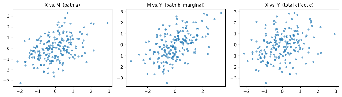

Step 2 — Estimate the paths with two regressions¶

Path analysis on observed variables reduces to a sequence of regressions:

Path $a$ — slope of $M \sim X$
Paths $c'$ and $b$ — slopes of $Y \sim X + M$ (the full model)
Path $c$ — slope of $Y \sim X$ (the reduced model, total effect)

The decomposition $c = c' + ab$ holds exactly for OLS estimates — the indirect effect $\widehat{a}\widehat{b}$ equals $\widehat{c} - \widehat{c'}$ to machine precision.

def ols(y, *preds):
    """OLS coefficients (intercept first) for y ~ 1 + preds."""
    D = np.column_stack([np.ones(len(y)), *preds])
    return np.linalg.lstsq(D, y, rcond=None)[0]

a_hat = ols(M, X)[1]              # M ~ X
cp_hat, b_hat = ols(Y, X, M)[1:3] # Y ~ X + M
c_hat = ols(Y, X)[1]              # Y ~ X

paths = pd.DataFrame(
    {"true":     [a_true, b_true, cp_true, cp_true + a_true * b_true, a_true * b_true],
     "estimate": [a_hat,  b_hat,  cp_hat,  c_hat,                     a_hat * b_hat]},
    index=["a (X->M)", "b (M->Y|X)", "c' (direct)", "c (total)", "a*b (indirect)"])
print(paths.round(3))

print(f"\nDecomposition check: c - c' = {c_hat - cp_hat:.6f}  vs  a*b = {a_hat * b_hat:.6f}")

                true  estimate
a (X->M)         0.6     0.519
b (M->Y|X)       0.5     0.531
c' (direct)      0.2     0.130
c (total)        0.5     0.406
a*b (indirect)   0.3     0.275

Decomposition check: c - c' = 0.275401  vs  a*b = 0.275401

All five quantities land near their true values, and $\widehat{c} - \widehat{c'} = \widehat{a}\widehat{b}$ exactly. In the CANlab Mediation Toolbox, mediation(X, Y, M, 'boot') returns these same five numbers as the columns of paths: [a b c' c a*b].

Step 3 — Bootstrap inference for the indirect effect¶

To test $H_0\!: ab = 0$ we need the sampling distribution of $\widehat{a}\widehat{b}$ . The product of two normal coefficients is not normal — it is skewed — which is why the normal-theory Sobel test is overconservative. The bootstrap sidesteps the approximation: resample participants with replacement, re-estimate $a \times b$ each time, and read the confidence interval and P value off the empirical distribution.

def boot_indirect(X, M, Y, n_boot=5000, seed=0):   # n_boot: ~5,000+ for stable CI tails
    """Percentile bootstrap distribution of the indirect effect a*b."""
    r = np.random.default_rng(seed)
    n = len(X)
    ab = np.empty(n_boot)
    for i in range(n_boot):
        idx = r.integers(0, n, n)              # resample cases with replacement
        ab[i] = ols(M[idx], X[idx])[1] * ols(Y[idx], X[idx], M[idx])[2]
    return ab

boot_ab = boot_indirect(X, M, Y)
lo, hi = np.percentile(boot_ab, [2.5, 97.5])
p_boot = 2 * min((boot_ab <= 0).mean(), (boot_ab >= 0).mean())

# Sobel test for comparison (normal-theory SE of the product)
def sobel(X, M, Y):
    n = len(X)
    a = ols(M, X)[1]
    se_a = np.sqrt(np.sum((M - ols(M, X)[0] - a * X) ** 2) / (n - 2) / np.sum((X - X.mean()) ** 2))
    D = np.column_stack([np.ones(n), X, M])
    beta = np.linalg.lstsq(D, Y, rcond=None)[0]
    resid = Y - D @ beta
    covb = np.sum(resid ** 2) / (n - 3) * np.linalg.inv(D.T @ D)
    b, se_b = beta[2], np.sqrt(covb[2, 2])
    z = a * b / np.sqrt(a**2 * se_b**2 + b**2 * se_a**2)
    return a * b, z, 2 * stats.norm.sf(abs(z))

ab_est, z_sobel, p_sobel = sobel(X, M, Y)
print(f"indirect a*b = {ab_est:.3f}")
print(f"bootstrap:  95% CI [{lo:.3f}, {hi:.3f}],  p = {p_boot:.4f}")
print(f"Sobel test: z = {z_sobel:.2f},  p = {p_sobel:.2e}")

plt.figure(figsize=(6, 3.5))
plt.hist(boot_ab, bins=60, color="steelblue", alpha=0.8)
plt.axvline(0, color="k", lw=1)
plt.axvline(lo, color="r", ls="--"); plt.axvline(hi, color="r", ls="--")
plt.xlabel("bootstrap $\\hat{a}\\hat{b}$"); plt.ylabel("count")
plt.title("Bootstrap distribution of the indirect effect")
plt.tight_layout(); plt.show()

indirect a*b = 0.275
bootstrap:  95% CI [0.177, 0.387],  p = 0.0000
Sobel test: z = 4.83,  p = 1.38e-06

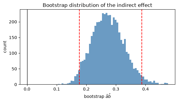
The confidence interval excludes zero decisively — as it should, since the data contain true mediation. Note the mild right skew of the bootstrap distribution: this is exactly the feature the Sobel normal approximation ignores. (The CANlab toolbox refines the percentile interval further with bias-corrected, accelerated bootstrapping.)

Step 4 — An unmodeled confounder creates spurious mediation¶

Now the cautionary tale. The causal interpretation of $a \times b$ requires no unmodeled confounding of the $M$ – $Y$ relationship. Randomizing $X$ protects paths $a$ and $c$ , but the mediator is only observed — so a lurking variable $U$ (say, general arousal) that raises both ACC activity and heart rate can create a $b$ path out of thin air.

We simulate a world with no true mediation at all: $M$ does not influence $Y$ ( $b = 0$ ). Instead, $U$ drives both.

# Ground truth: X affects M and Y, but M has NO effect on Y (b = 0).
# A confounder U (e.g., arousal) affects both M and Y.
U  = rng.standard_normal(n)
M2 = 0.6 * X + 0.7 * U + rng.standard_normal(n)          # a = 0.6, confounded
Y2 = 0.3 * X + 0.0 * M2 + 0.7 * U + rng.standard_normal(n)  # true b = 0 !

# Naive mediation analysis (U unmeasured / ignored):
boot_naive = boot_indirect(X, M2, Y2, seed=1)
lo1, hi1 = np.percentile(boot_naive, [2.5, 97.5])
ab_naive = ols(M2, X)[1] * ols(Y2, X, M2)[2]
print(f"NAIVE  : a*b = {ab_naive:.3f}, 95% CI [{lo1:.3f}, {hi1:.3f}]"
      f"  ->  {'SPURIOUS mediation!' if lo1 > 0 or hi1 < 0 else 'ns'}")

# Correct analysis: include U as a covariate in both path regressions
a_adj  = ols(M2, X, U)[1]
b_adj  = ols(Y2, X, M2, U)[2]
r2 = np.random.default_rng(2)
boot_adj = np.empty(5000)
for i in range(5000):
    idx = r2.integers(0, n, n)
    boot_adj[i] = ols(M2[idx], X[idx], U[idx])[1] * ols(Y2[idx], X[idx], M2[idx], U[idx])[2]
lo2, hi2 = np.percentile(boot_adj, [2.5, 97.5])
print(f"ADJUSTED for U: a*b = {a_adj * b_adj:.3f}, 95% CI [{lo2:.3f}, {hi2:.3f}]"
      f"  ->  {'still significant' if lo2 > 0 or hi2 < 0 else 'no mediation (correct!)'}")

NAIVE  : a*b = 0.199, 95% CI [0.112, 0.304]  ->  SPURIOUS mediation!
ADJUSTED for U: a*b = -0.000, 95% CI [-0.076, 0.079]  ->  no mediation (correct!)

The naive analysis “detects” a significant indirect effect even though $M$ has zero causal effect on $Y$ : the confounder induces an $M$ – $Y$ partial correlation, and the machinery happily multiplies it by $a$ . Adding $U$ as a covariate (the 'covs' option in mediation.m) recovers the truth. In real data $U$ is usually unmeasured — which is why the chapter frames fMRI mediation as pathway discovery, not causal proof.

Step 5 — A three-node path model fit by regression equations¶

Finally, the recursive SEM of Figure 34.1: ROI 1 drives ROIs 2 and 3 ( $b_{12}$ , $b_{13}$ ), and ROI 2 drives ROI 3 ( $b_{23}$ ). In matrix form $y = B y + \zeta$ , and because the model is recursive (no loops), each equation can be estimated by OLS:

ROI 2 $\sim$ ROI 1 $\;\Rightarrow\; b_{12}$
ROI 3 $\sim$ ROI 1 + ROI 2 $\;\Rightarrow\; b_{13}, b_{23}$

We then rebuild $B$ , form the model-implied covariance $\Sigma(\theta) = (I-B)^{-1}\Psi(I-B)^{-T}$ , and compare it with the sample covariance — the quantity SEM software minimizes. (Note the mediation model of Steps 1–3 is exactly this graph with ROI 1 = $X$ , ROI 2 = $M$ , ROI 3 = $Y$ .)

# Simulate T time points from the recursive path model (true edges below)
T = 300                                      # T = time points in the simulated series
b12_true, b13_true, b23_true = 0.8, 0.4, 0.5 # true path coefficients for the three edges

z = rng.standard_normal((3, T))          # independent errors zeta, unit variance
y1 = z[0]
y2 = b12_true * y1 + z[1]
y3 = b13_true * y1 + b23_true * y2 + z[2]
Ydat = np.vstack([y1, y2, y3])           # 3 x T

# Fit each structural equation by OLS
b12_hat = ols(y2, y1)[1]
b13_hat, b23_hat = ols(y3, y1, y2)[1:3]
print(f"path estimates: b12 = {b12_hat:.3f} (true {b12_true}), "
      f"b13 = {b13_hat:.3f} (true {b13_true}), b23 = {b23_hat:.3f} (true {b23_true})")

# Rebuild B and the model-implied covariance Sigma = (I-B)^-1 Psi (I-B)^-T
B = np.array([[0,       0,       0],
              [b12_hat, 0,       0],
              [b13_hat, b23_hat, 0]])
resid_var = np.array([np.var(y1, ddof=1),
                      np.var(y2 - b12_hat * y1, ddof=2),
                      np.var(y3 - b13_hat * y1 - b23_hat * y2, ddof=3)])
Psi   = np.diag(resid_var)
IminB = np.eye(3) - B
Sigma_model = np.linalg.inv(IminB) @ Psi @ np.linalg.inv(IminB).T
Sigma_obs   = np.cov(Ydat)

print("\nobserved covariance:\n", Sigma_obs.round(3))
print("model-implied covariance:\n", Sigma_model.round(3))
print(f"max |difference| = {np.abs(Sigma_obs - Sigma_model).max():.4f}")

path estimates: b12 = 0.788 (true 0.8), b13 = 0.414 (true 0.4), b23 = 0.489 (true 0.5)

observed covariance:
 [[1.116 0.879 0.892]
 [0.879 1.742 1.216]
 [0.892 1.216 1.911]]
model-implied covariance:
 [[1.116 0.879 0.892]
 [0.879 1.746 1.218]
 [0.892 1.218 1.918]]
max |difference| = 0.0072

The model-implied and observed covariances agree almost perfectly — with 3 variables and 6 free parameters (3 paths + 3 error variances) matching 6 covariance moments, this model is just-identified: it can always reproduce the data covariance, so overall fit cannot be tested. Fit tests need over-identified models with fewer parameters than moments.

We can, however, test an individual edge by model comparison: does the direct ROI 1 → ROI 3 connection ( $b_{13}$ ) improve the model beyond the indirect route through ROI 2? Dropping the edge gives a nested model, and for a single OLS-estimated path this likelihood-ratio-style comparison reduces to the familiar t-test on $b_{13}$ .

# Test the ROI1 -> ROI3 edge: full model (y3 ~ y1 + y2) vs. reduced (y3 ~ y2)
D_full = np.column_stack([np.ones(T), y1, y2])
D_red  = np.column_stack([np.ones(T), y2])
beta_f = np.linalg.lstsq(D_full, y3, rcond=None)[0]
sse_f  = np.sum((y3 - D_full @ beta_f) ** 2)
beta_r = np.linalg.lstsq(D_red, y3, rcond=None)[0]
sse_r  = np.sum((y3 - D_red @ beta_r) ** 2)

F  = (sse_r - sse_f) / 1 / (sse_f / (T - 3))     # nested model comparison
pF = stats.f.sf(F, 1, T - 3)
print(f"edge b13: F(1, {T - 3}) = {F:.2f}, p = {pF:.2e}"
      f"  ->  the direct ROI1->ROI3 connection {'improves' if pF < .05 else 'does not improve'} the model")

edge b13: F(1, 297) = 36.20, p = 5.22e-09  ->  the direct ROI1->ROI3 connection improves the model

Wrap-up¶

You built the full path-modeling toolkit for observed variables: estimating path coefficients with regressions, decomposing total effects into direct and indirect parts, bootstrapping the skewed product $a \times b$ , and testing edges by nested model comparison against the model-implied covariance. You also saw the framework’s Achilles heel — an unmodeled $M$ – $Y$ confounder is indistinguishable from true mediation in observational data.

In MATLAB, the CANlab Mediation Toolbox wraps this workflow in mediation.m (with bias-corrected bootstrap, robust regression, multilevel models, and moderated mediation) and scales it to whole-brain search with mediation_brain.m. Return to the chapter page for the conceptual context, and see Chapter 35 for dynamic causal models, which build directionality into a biophysical generative model rather than a covariance structure.