Day 2 · Modeling, connectivity, and ICA

Day 2Session 2.1Wager0:30 hLecture

GLM model building: predictors and contrasts

This session moves from a single-regressor GLM to designs with multiple event types, and introduces contrasts as the tool for testing differences, averages, and custom hypotheses on the fitted betas. It sets out the two practical rules for T-contrasts, an expected value of zero under the null and consistent scaling, and explains why scaling matters when contrast images are carried to a group analysis, especially when participants have missing runs.

Take-aways

  • Model each event type separately in event-related designs, then use contrasts to test differences, averages, or custom hypotheses.
  • Contrasts testing differences should sum to zero; tests against the implicit baseline are the exception.
  • Use the same weights for every participant and scale positive and negative weights to sum to +1 and -1 so missing runs do not change the contrast scale.

Key terms

  • contrast
  • contrast weight vector (c)
  • T-contrast
  • ANOVA contrast
  • planned comparison
  • implicit baseline
  • con image
  • contrast scaling
  • missing runs
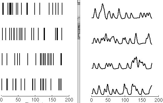
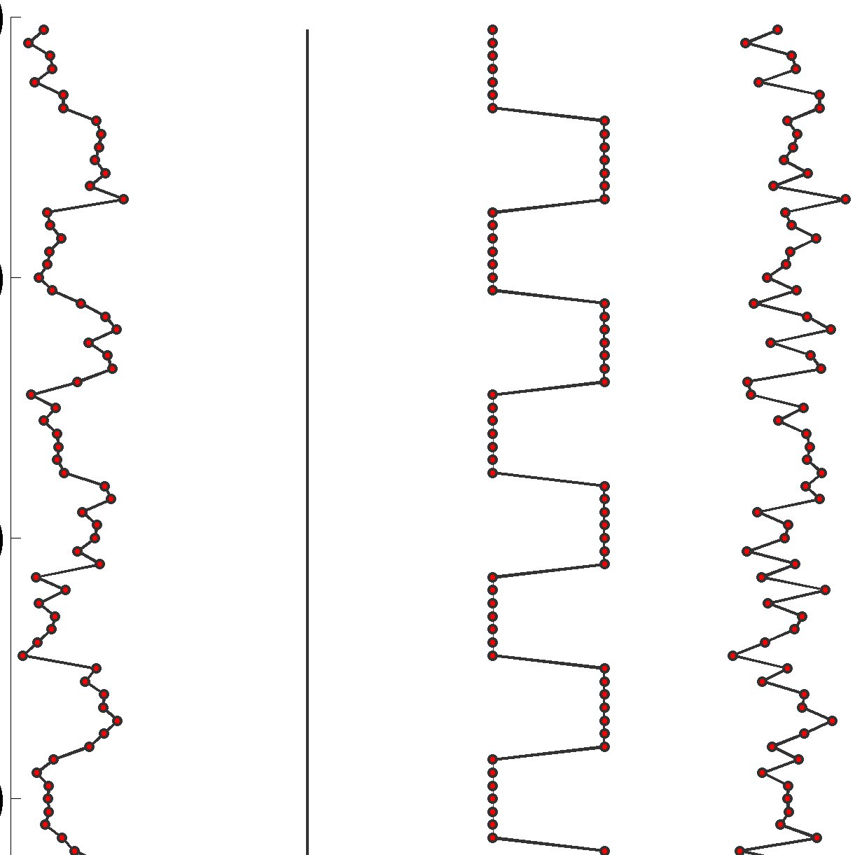
Observed data, box-car predictor, and residual noise over time
Observed data, box-car predictor, and residual noise over time. Lecture 2.1 slides (Wager)

Outline

What the session covers

01From single-predictor to multiple-predictor designs

  • Famous vs. non-famous faces example: the question is a difference between two conditions.
  • In a block design a single regressor can directly capture the famous-minus-non-famous difference.
  • Basic first-level design matrix: an intercept plus a task regressor, with betas as slopes and residuals left over.
  • In event-related designs, model each event type as its own regressor.
  • With separate regressors you can test the difference, each condition alone, or their average, each via a different linear contrast.

02Contrasts as a flexible tool

  • A contrast is a linear combination of GLM parameters, specified by a weight vector c so that c-transpose-beta is a scalar.
  • A T-contrast is a single planned comparison tested with a t-test; weights are signed (positive or negative).
  • ANOVA-style contrasts express planned comparisons, e.g., weights [1 1 -1 -1] give the main effect (A+B) minus (C+D).
  • C can be a matrix; each column is applied independently and is a separate test.
  • Custom contrasts are not limited to ANOVA effects; specify whatever planned tests follow from your hypotheses.
Stick-function event onsets and their HRF-convolved regressors
Stick-function event onsets and their HRF-convolved regressors. Lecture 2.1 slides (Wager)
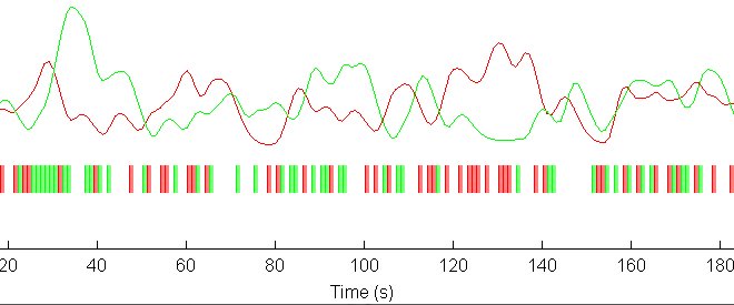
Two-condition predicted BOLD time courses with event onsets
Two-condition predicted BOLD time courses with event onsets. Lecture 2.1 slides (Wager)

03Rule 1: expected value must be zero under the null

  • Null hypothesis is c-transpose-beta = 0, alternative is not equal to 0, which permits a t-test.
  • When testing a difference between conditions, the contrast weights should sum to zero.
  • Exception: testing the average of one or more conditions against the implicit baseline, e.g., H0: (betaA + betaB)/2 = 0.
  • This works because regression betas are signed and zero under the null, so testing against zero is reasonable.

04Rule 2: scaling of contrast weights

  • For a single subject, weight scaling changes the contrast magnitude but not t- or p-values; [1 -1] and [.5 -.5] are equivalent.
  • In imaging, contrast magnitudes (con images) go to group analysis, so scale must be comparable across participants.
  • Contrast weights must be the same for all participants; beware of missing sessions or runs.
  • Summing across three runs ([1 1 1]) is not equivalent to summing across four; the scale becomes 3*(F-N) vs. 2*(F-N) even with identical activation.
  • Fix: scale so the contrast is mean(F) minus mean(N) across runs, i.e., positive weights sum to +1 and negative weights sum to -1.
  • Consistent scaling also supports interpreting contrast values on a meaningful scale such as percent signal change.
ICA component maps with time courses on brain slices — Lecture 2.10 slides (Calhoun)

From the instructors' research

Related figures

Examples of these concepts in published work by the course instructors.

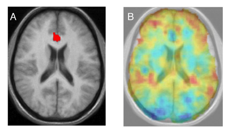
Region of interest and estimated HRF amplitude map
Region of interest and estimated HRF amplitude map. Lindquist et al. (2009), NeuroImage
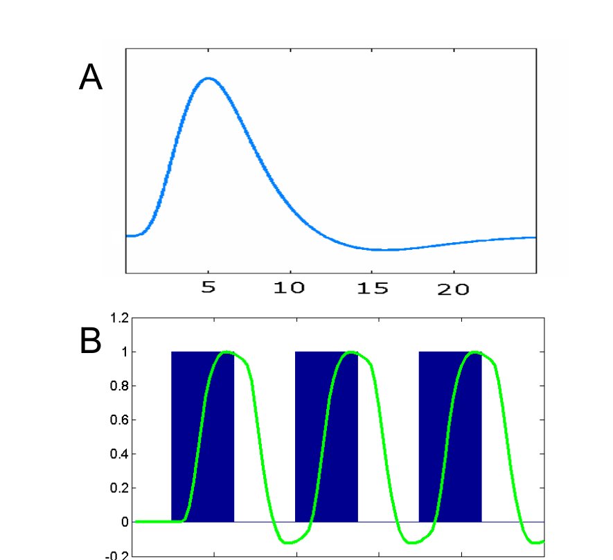
Canonical hemodynamic response and block convolution
Canonical hemodynamic response and block convolution. Lindquist & Wager (2014), Principles of fMRI (book chapter)