Day 2 · Modeling, connectivity, and ICA

Day 2Session 2.10Calhoun1:30 hLecture

Introduction to ICA: Independent Component Analysis

This session introduces independent component analysis as a data-driven alternative to seed-based and GLM approaches for fMRI. It covers the blind source separation model, the difference between ICA and PCA, spatial ICA of fMRI and the kinds of components it yields, the sorting and scaling ambiguities, model-order selection, validation strategies, and available software including the GIFT toolbox.

Take-aways

  • ICA decomposes fMRI data into spatially independent maps and their time courses without a model of the time course, unlike the GLM or seed correlation.
  • Components must be sorted and calibrated because ICA solutions are ambiguous up to permutation and scale.
  • Model order, algorithm, and preprocessing all affect results; use information criteria, ICASSO-style clustering, and validation with known sources.

Key terms

  • independent component analysis
  • blind source separation
  • mixing matrix
  • non-Gaussianity
  • Infomax
  • FastICA
  • spatial ICA
  • permutation and scaling ambiguity
  • model order (AIC/MDL)
  • GIFT
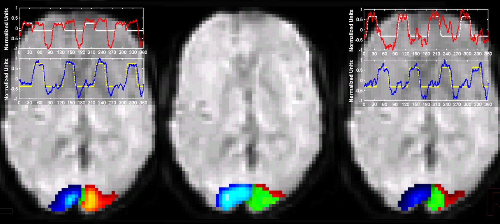
ICA component maps with associated time courses on brain slices
ICA component maps with associated time courses on brain slices. Lecture 2.10 slides (Calhoun)

Outline

What the session covers

01Motivation: seeds versus components

  • 'All models are wrong, but some are useful' (Box); data-driven methods play to our ignorance about the right model.
  • Seed approaches need one or more seed regions, univariate cross-correlation, filtering, physiological noise removal, and a decision between full and partial correlation.
  • ICA is fully data-driven (no seed, though priors are possible), assumes linear covariation within and linear mixing among components, and maximizes spatial independence.
  • All components have values at every voxel, enabling spatial filtering of artifacts and overlapping components.
  • 'Network' depends on method: correlation with a reference signal (GLM, seeds), with a component time course (ICA), or a connectivity matrix (graph theory).
02ICA basics

  • Blind source separation (cocktail party problem): recover sources from mixed observations without knowing the mixing.
  • Model X = A S (mixture, mixing matrix, sources); estimate the unmixing matrix W = A^-1 so that S = W X.
  • Assumptions: linear mixing, statistically independent sources, and non-Gaussian sources.
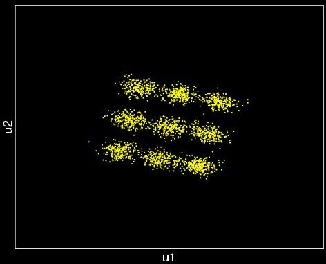
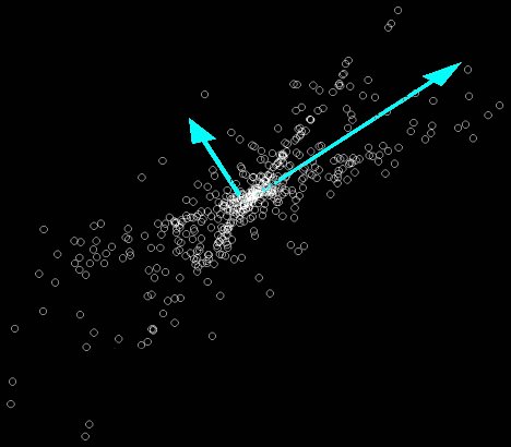
  • PCA finds directions of maximal variance using second-order statistics; ICA finds directions maximizing independence using higher-order statistics.
  • Algorithm families: Infomax (Bell and Sejnowski 1995), maximum likelihood, negentropy/FastICA (Hyvarinen), minimum mutual information, JADE; Infomax equals ML when the nonlinearity matches the cdf.
  • ICA maximizes non-Gaussianity; many real signals are supergaussian (peaked with heavy tails), and the FastICA demo shows whitening followed by iterative rotation.
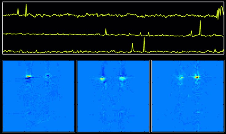
ICA component time courses and their spatial maps
ICA component time courses and their spatial maps. Lecture 2.10 slides (Calhoun)
PCA directions on a scatter of mixed sources
PCA directions on a scatter of mixed sources. Lecture 2.10 slides (Calhoun)

03ICA of fMRI

  • The GLM requires a model for the fMRI time course; spatial ICA estimates the time courses along with the source locations.
  • Data (time by voxels) equals a mixing matrix of time courses multiplied by spatially independent component maps.
  • Typical components: task-related, cardiac, motion (e.g., mouth movement in inferior temporal and orbitofrontal regions), vasomotor oscillation and high-order visual.
  • ICA is useful for artifact detection and reduction (Beckmann's 'Little Shop of fMRI Horrors'); preprocessing may differ when hunting artifacts.
  • Spatial ICA is more common than temporal ICA; results differ when components are spatially dependent.
  • ICA is not model-free, but it assumes nothing about time-course shape; data-driven does not mean fishing, and tools exist for focused questions.

04Sorting and calibration

  • Permutation ambiguity, X = (A P^-1)(P S), means component order is arbitrary, so sorting is needed.
  • Scaling ambiguity, X = (A M^-1)(M S), means amplitudes are arbitrary, so calibration is needed.
  • Temporal sorting: correlation or multiple regression with a design, or features such as skew, kurtosis, and power spectra.
  • Spatial sorting: correlation with a mask or SPM map, maximum value within a mask, multiple regression.
  • Multivariate sorting and classification: SVM approaches (Formisano), Noisecloud (Sochat), FSL-FIX (Griffanti).
Unmixed ICA source clusters
Unmixed ICA source clusters. Lecture 2.10 slides (Calhoun)

05Number of components (model order)

  • Too many components over-split; too few over-clump.
  • Between 20 and 40 is reasonable for a typical experiment, but many studies now use higher orders (75-200).
  • Order is estimated from PCA eigenvalues with AIC, MDL, or BIC; MDL is consistent, AIC may do better at low SNR (correlated-sample correction: Li 2006).
  • Post-ICA clustering is another way to address model order, and low-order components can be reconstructed from higher-order decompositions.

06Validation and software

  • Validation studies address algorithm differences (Esposito 2002), preprocessing (Calhoun 2004), cluster validation via ICASSO (Himberg 2004), and test-retest performance (Nybakken 2002).
  • Hybrid experiments mix known sources into real fMRI data and score recovery with Kullback-Leibler divergence; Infomax was consistent across runs (Correa et al. 2006).
  • Packages: GIFT (over 15 algorithms, constrained ICA, sorting and visualization, dynamic connectivity, batch scripting), MELODIC in FSL, FMRLAB, ICALAB, BrainVoyager, DTU toolbox.
  • GIFT has over 25,000 unique downloads and a BIDS-App (GIFTBIDS).
  • GIFT BIDS-App demo: install Docker, download the demo dataset, copy config_multi_ses.m, and run the trends/gift-bids container with --participant_label and --config.
PINES negative-affect signature rendered on cortical surfaces — Chang et al. (2015), PLoS Biology

From the instructors' research

Related figures

Examples of these concepts in published work by the course instructors.

Simulated spatial component map for group ICA
Simulated spatial component map for group ICA. Allen et al. (2012), NeuroImage
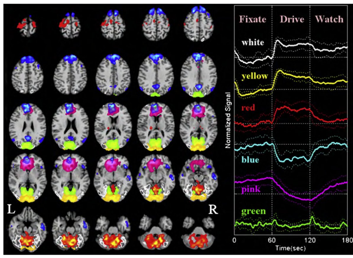
Multiple networks identified during simulated driving
Multiple networks identified during simulated driving. Calhoun et al. (2009), NeuroImage