Autocorrelation and generalized linear models

This session covers temporal autocorrelation in fMRI noise, why it violates the independence assumption of ordinary least squares, and how generalized least squares with prewhitening addresses it. It describes autoregressive noise models, the iterative estimation procedure used in SPM (ReML via EM), differences among SPM, AFNI, and FSL, and practical guidance on when autocorrelation modeling matters.

Scroll down

Take-aways

fMRI errors are autocorrelated, so OLS p-values and degrees of freedom are wrong for single-subject inference.
Prewhitening with an iteratively estimated AR or ARMA model (ReML via EM in SPM) restores valid inference when the noise model fits.
Choose the simplest adequate noise model; FAST or ARMA(1,1) generally outperform AR(1), and group analyses do not require autocorrelation modeling.

Key terms

temporal autocorrelation
white noise
AR(1) model
ARMA(1,1)
sphericity
generalized least squares (GLS)
prewhitening
Yule-Walker
ReML
FAST

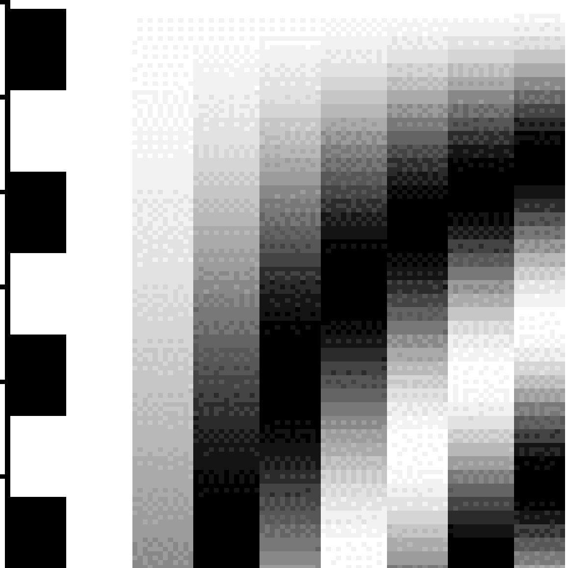
**Discrete cosine basis set beside a box-car task regressor.** Lecture 2.8 slides (Wager)

Outline

What the session covers

01Types of noise

Post-acquisition options: remove noise (high-pass filtering, physiological models) or model its structure (autocorrelation, multilevel); the first helps more.
White noise: independent errors, flat power spectrum, no temporal correlation.
Structured noise arises from identifiable processes; stationary noise has constant mean, variance, and autocorrelation, nonstationary noise does not.
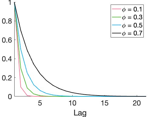
AR noise: carry-over of noise from previous time points, stationary; AR(1) is epsilon_t = phi * epsilon_(t-1) + eta_t, with higher phi meaning more autocorrelation.
Brownian (random walk) noise integrates independent innovations and is nonstationary, with variance growing over time.
1/f-like noise falls in power with frequency; AR models capture geometric decay of carry-over, MA terms capture non-propagating carry-over, and ARMA(1,1) includes both.

02Modeling approaches and software

Three options: assume independence (ignore), precoloring (SPM99 temporal smoothing), or prewhitening (preferred).
Prewhitening uses iterative estimation of the noise structure: AR(1) (SPM5), AR(1) plus white noise, ARMA(1,1).
SPM: AR(1) linear approximation, or FAST (linearization of an exponential); AFNI: ARMA(1,1); FSL: arbitrary autocorrelation function with a Tukey taper.
Estimation requires the variance, the AR phi parameter, and the degrees of freedom, via an iterative procedure (Box, Jenkins and Reinsel).

**AR(1) autocorrelation functions for several phi values.** Lecture 2.8 slides (Wager)

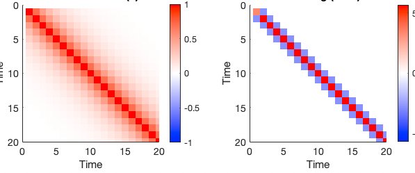
**Autocorrelation matrix and its whitening matrix.** Lecture 2.8 slides (Wager)

03The error covariance matrix and whitening

GLM: Y = X beta + epsilon with cov(epsilon) = V; OLS assumes sphericity, V = sigma^2 I.
Violations of sphericity: serial autocorrelation (AR(1) form with rho, rho^2, rho^3 off the diagonal), unequal variances, and repeated-measures covariance.
Whitening multiplies the data and design by a matrix derived from the inverse error covariance to decorrelate the time series.
Iteration: start with W = I (OLS), compute residuals, estimate sample autocovariance, fit AR parameters (Yule-Walker), build the whitening matrix, re-estimate betas.
The independence model versus an AR model really does make a difference to the resulting statistics.
ReML (restricted maximum likelihood) maximizes the likelihood of the residuals and gets degrees of freedom right; SPM finds ReML variance parameters with expectation maximization (EM).

04Choosing an autocorrelation model

Aim for the simplest model that accurately describes the noise structure.
Complex models are more accurate with large, clean datasets but less precise with limited data; n = 500 simulations show more error variability.
FAST in SPM decomposes residual covariance into exponential and derivative terms and outperformed SPM AR(1) and FSL in several large datasets (Olszowy 2019).
Autocorrelation modeling is not needed for group analysis; it is needed for single-subject inference, which is often fragile anyway because of artifacts.
SPM2 through SPM12 use an AR(1) approximation pooled across the brain, which only helps if the AR model fits the data well.
FAST in SPM or AFNI's ARMA(1,1) is preferred to AR(1) or FSL's ACF in many cases; BROCCOLI uses voxelwise AR(4) by default.

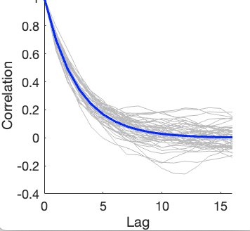
**Flexible autocorrelation estimates across voxels with mean curve.** Lecture 2.8 slides (Wager)

05Summary: issues in using the GLM for fMRI

Unknown neural response shape: assume one (event or epoch).
Delayed, dispersed BOLD response: use an HRF.
HRF shape varies across the brain: use basis functions.
Low-frequency noise and motion or cardiopulmonary artifacts: high-pass filter and model known noise sources.
Temporal autocorrelation violates GLM assumptions: use iterative autocorrelation models, or focus on group statistics and ignore it.

Tissue segmentation of axial brain slices in warm and cool tones — Lecture 2.2 slides (Wager)

Previous · 2.7Parametric modulators Next · 2.9Intro to connectivity and mediation; mediation demo/walkthrough

Day 2 · Modeling, connectivity, and ICA

2.1 GLM model building: predictors and contrasts 2.2 GLM filtering and nuisance regressors 2.3 GLM multicollinearity and diagnostics 2.4 SPM GUI for single subjects: explore design, scaling, results 2.5 Basis sets: flexible hemodynamic modeling 2.6 Derivative boost 2.7 Parametric modulators2.8 Autocorrelation and generalized linear models2.9 Intro to connectivity and mediation; mediation demo/walkthrough 2.10 Introduction to ICA: Independent Component Analysis